Backstepping Technique Based on Error

Li Wang

School of Hydraulic, Energy and Power Engineering, Yangzhou University, Yangzhou, China.

DOI: 10.4236/oalib.1103061                

Abstract

Backstepping technique usually adopts back step design to construct the Lyapunov function gradually, and then to design the corresponding virtue controller. The backstepping technique based on error also adopts back step design process, but the design of virtue controllers depends on the corresponding errors which are designed to satisfy some expected behaviors. Six different error equations are deduced by changing the results of the virtue controls arbitrarily while guaranteeing the system behaviors such as stability, and an example shows the effectiveness of these six versions. Simulated results illustrate that these six versions of backstepping technique based on error are effective.

Keywords

Backstepping Technique, Lyapunov Function, Error, Strictly Feedback Nonlinear Control System

1. Introduction

A new redesign backstepping technique, backstepping technique based on error is presented in this paper, which also adopts backstepping design process, but doesn’t construct the system, control Lyapunov function; the design of the virtue controller depends on the corresponding errors which are designed to satisfy some expected behaviors. The method is also more flexible than DSC. Based on some results of [13] , we deduce six different error equations by changing the result of the virtue control law arbitrarily while guaranteeing the system behaviors such as stability.

In this paper, we call backstepping technique based on control Lyapunov functions as conventional backstepping, and call backstepping technique based on error as error backstepping. Section 2 presents the design and six results of error backstepping, in Section 3 an example shows the effectiveness of these six versions, and Section 4 concludes this paper.

2. Backstepping Technique Based on Error

Consider a usual strictly feedback nonlinear system as follows:

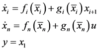(1)

where, , when , ,. The design objective is to make.

The backstepping design process is as follows.

Step 1: Consider the control goal, take as the first virtual control and pretend that satisfies the following equation.

(2)

Define the first tracking error

(3)

Error is wanted to converge to zero exponentially, therefore select the desired behaviour to be is chosen to satisfy the required dynamic characteristic.

(4)

Then the following equality corresponds to desired behaviour

(5)

Step 2: but we cannot just choose to be, so we “step back” one integrator to the equation. Choose as the second virtual control to solve the tracking problem.

Introduce

(6)

Define the second tracking error:

(7)

The error is also wanted to converge to zero exponentially, and select the desired behaviour to be:

(8)

is chosen to satisfy the required dynamic characteristic.

(9)

Then the following equality corresponds to desired behavior.

(10)

Step i: Choose as the i virtual control to solve the tracking problem. Define the i tracking error

(11)

Select its time derivative to satisfy the following behaviou

(12)

Introduce

(13)

Choose to satisfy the required behaviour

(14)

Then has

(15)

Step n: Choose u to solve the tracking problem. Define the n tracking error:

(16)

Its derivative satisfies.

In fact:

(17)

The last equality corresponds to what we are forcing.

(18)

The deduced error equation is:

(19)

Defining, then

(20)

Proposition 2.1: When choose parameters

and

where is constant. It is obvious that errors converge to origin exponentially, that is,.

Proposition 2.2: When is the function of, and when select appropriate parameters, It can make errors globally stable at origin, then.

Proof: error Equation (19) is in short as, where

(21)

Introduce

(22)

Its time derivative is

(23)

If parameters satisfy, , , , , then, so all the errors converge to origin globally.

End of proof.

Proposition 2.3: Assume the expression of virtual control (14) is changed into:

(24)

where, when choose the parameters and is the function of the corresponding states, errors converge to origin globally, and,.

Proof: when virtual control (24) takes place (14) in recursive procedure, the new error equation is changed into

or

(25)

It is the same as (2.27). Then all the errors converge to origin globally.

End of proof.

Proposition 3.4: Similarly assume the expression of virtual control (8) is changed into:

(26)

where, , and is the function of the corresponding states, then the new error equation is:

or

(27)

When choose the parameters and, errors are globally asymptotically stable at origin, and.

Proof:

Defining

(28)

where

(29)

Then

(30)

Introduce a positive definite quadratic function

(31)

It can be obtained

(32)

Then converge to origin globally, so errors are globally asymptotically stable at origin and.

End of proof.

Proposition 2.5: The virtual control can also be choose as

(33)

where, , and is the function of the corresponding states, then the new error equation is:

or

(34)

When choose parameters and the following inequality is satisfied

(35)

Errors c are globally asymptotically stable at origin, and .

Proof:

Define as follows:

(36)

Then it can be obtained

(37)

where

(38)

(39)

Introduce a positive definite function, where is chosen as, then, where, then the time derivative of is

(40)

Because

(41)

So

(42)

It is obvious that is a diagonal matrix, and the i diagonal unit is, from (35) and (36), we deduced that

(43)

Substituting (42) into (43), it can be deduced that is negative definite, so errors converge to origin globally.

End of proof.

Proposition 2.6: The virtual control can also be choose as

(44)

where, , and is the function of the corresponding states, then the new error equation is:

or

(45)

When choose parameters and the following inequality is satisfied

(46)

Errors are globally asymptotically stable at origin, and .

Proof: it is similar to the proof of Proposition 2.5.

3. Numerical Simulation

Consider the following two-order system:

(47)

The control objective is to design a state feedback control to asymptotically stabilize the origin.

We adopt backstepping technique based on error to design control law. The calculated results are presented in Table 1 by choosing parameters. If the initial conditions are, the simulated results are shown in Figure 1.

As it is shown in Figure 1 the transients of state variables and error variables are stable, they get to origin in finite time. It is also shown that when the system structure or the control law is simple the transients of state variables and converge to origin perfectly.

Table 1. Calculated results.

Figure 1. Simulated results.

4. Conclusion

The backstepping technique based on error is the expansion of the backstepping technique, it adopts backstepping design process, but the design of the virtue controller depends on the corresponding errors which are designed to satisfy some expected behaviors. This method makes the design systematical and structural, and it can change the result of the virtue control law arbitrarily in six forms while guaranteeing the system stability. The method can be used for both stabilization control problems and tracking control problems. Subjects of future research include the discussions of systems that contain uncertain terms, unknown parameters or unmeasured signals.

Conflicts of Interest

The authors declare no conflicts of interest.

References

[1]	Kanellakopoulos, I., Kokotovic, P.V. and Morse, A.S. (1991) Systematic Design of Adaptive Controllers for Feedback Linearizable Systems. IEEE Transactions on Automatic Control, 36, 1241-1253.
[2]	Kovotovic, P.V. (1992) The Joy of the Feedback: Nonlinear and Adaptive. IEEE Control System, 12, 7-17.
[3]	Kokotovic, P.V., Krstic, M. and Kmellakopoulos, I. (1992) Backstepping to Passivity: Recursive Design of Adaptive Systems. Proceedings of the 31st Conference on Decision & Control, Tucson, 16-18 December 1992, 3276-3280.
[4]	Krstic, M., Kanellakopoulos, I. and Kokotovic, P.V. (1995) Nonlinear and Adaptive Control Design. John Wiley & Sons, New York.
[5]	Arcak, M., Seron, M., Braslavsky, J. and Kokotovic, P.V. (2000) Robustification of Backstepping against Input Unmodeled Dynamics. IEEE Transactions on Automatic Control, 45, 1358-1363. http://dx.doi.org/10.1109/9.867048
[6]	Kokotovic, P. and Arcak, M. (2001) Constructive nonlinear control: A Historical Perspective. Automatica, 37, 637-662. http://dx.doi.org/10.1016/S0005-1098(01)00002-4
[7]	Dacic, D.B. and Kokotovic, P.V. (2005) A Scaled Feedback Stabilization of Power Integrator Triangular Systems. Systems & Control Letters, 54, 645-653. http://dx.doi.org/10.1016/j.sysconle.2004.11.004
[8]	Karagiannis, D. and Astolfi, A. (2008) Nonlinear Adaptive Control of Systems in Feedback Form: An Alternative to Adaptive Backstepping. Systems & Control Letters, 57, 733-739. http://dx.doi.org/10.1016/j.sysconle.2008.02.006
[9]	Tee, K.P., Ge, S.S. and Tay, E.H. (2009) Barrier Lyapunov Functions for the Control of Output-Constrained Nonlinear Systems. Automatica, 45, 918-927. http://dx.doi.org/10.1016/j.automatica.2008.11.017
[10]	Swaroop, D., Hedrick, J.K., Yip, P.P. and Gerdes, J.C. (2000) Dynamic Surface Control for a Class of Nonlinear Systems. IEEE Transactions on Automatic Control, 45, 1893-1899. http://dx.doi.org/10.1109/TAC.2000.880994
[11]	Chen, L. and Pan, C.P. (2009) Dynamic Surface Backstepping Control Design for One Hypersonic Vehicle. Proceedings of the 2009 IEEE International Conference on Mechatronics and Automation, Changchun, 9-12 August 2009, 4770-4774. http://dx.doi.org/10.1109/ICMA.2009.5246455
[12]	Song, B. (2006) Decentralized Dynamic Surface Control for a Class of Interconnected Nonlinear Systems. Proceedings of the 2006 American Control Conference, Minneapolis, 14-16 June 2006, 130-135. http://dx.doi.org/10.1109/ACC.2006.1655342
[13]	Liu, B. and Zhang, Z.K. (2007) Stability of Nonlinear Systems with Tridiagonal Structure and Its Application. Acta Automatica Sinica, 33, 442-445.