Approximate Solutions to the Discontinuous Riemann-Hilbert Problem of Elliptic Systems of First Order Complex Equations ()
1. Introduction
Let  be an
be an  -connected bounded domain in
  with the boundary
 . Without loss of generality, we assume that
  is a circular domain in
 , bounded by the
  -circles
  and
and . In this article, the notations are the same as in references [1] -[12] . If the first order elliptic system with
  unknown real functions
 (1.1)
(1.1)
satisfies certain conditions, then (1.1) can be transformed into the complex form
 (1.2)
(1.2)
where  (see Section 4, Chapter 2 in [5] ). Its vector form is as follows:
 (1.3)
(1.3)
where  is the transposed matrix of
 . We discuss the first order complex system (1.3) in the form
 (1.4)
(1.4)
in which  with
with ,
,  with
with 
 with
with 

We assume (1.4) satisfies the following conditions:
Condition C 1)  are continuous in
  for almost every point
2) The above functions are measurable in  for all systems of continuous functions
  in
in  and any systems of measurable functions
  in
in  and satisfy
 (1.5)
(1.5)
 (1.6)
(1.6)
where  is as stated in (1.8) below,
  and
and  are non-negative constants.
3) The complex system (1.4) satisfies the following ellipticity condition
 (1.7)
(1.7)
where  are non-negative constants.
For convenience,  and
and  are used to indicate
  and
and  respectively,
  and we define the following:

in which  and
and  are stated as in (1.12), (2.1) below, and
 and
and  are non-negative constants.
The so-called Riemann-Hilbert boundary value problem for the complex system (1.4) may be formulated as follows.
Problem A Find a system of continuous solutions  in
in  of (1.4), which satisfies the boundary condition
 (1.8)
(1.8)
in which  with
with  for
for 
 and
and
 are the first kind of discontinuous points of
  on
on .
.
Denote by  and
and  the left limit and right limit of
  as
as  on
on , and
, and
 (1.9)
(1.9)
where  when
when , and
, and  when
when . There is no harm in assuming that the partial indexes
  of
of  on
on  are not integers, and the partial indexes
  of
of  on
on  are integers. Set
 (1.10)
and we call  the index of Problem A.
For problem A, we will assume  satisfy the conditions
 (1.11)
in which  is an open arc from the point
  to
to  on
on 

 are non-negative constants,
 . Moreover, we require that the solution
  possess the property
 (1.12)
in , where
  in
in  and
and  are small positive constants.
In general, Problem A may not be solvable. Hence we propose a modified problem as follows.
Problem B Find a system of continuous solutions  of the complex equation (1.4) in
 , which satisfies the modified boundary condition
 (1.13)
Here
 (1.14)
in which 
 are unknown real constants to be determined appropriately, and
 , if
, if  is an odd integer. More description on
  and
and  are given below. We begin with the following function

where  denotes the partial index on
 ,
,  are fixed pointswhich are not the discontinuous points from
 . Note that the positive direction applies to the boundary circles
 . Similarly to (1.7)-(1.12), Chapter V, [2] , we see that

Clearly, with certain modification on the symbols on some arcs on ,
,  on
on  is seen to be continuous. In this case, its index

are integers. And we have the following:

in which  are solutions of the modified Dirichlet problems with the above boundary conditions for analytic functions,
  are real constants, and
 .
.
In addition, we may assume that the solution  satisfies the following point conditions
 (1.15)
where  are distinct points, and
  are all real constants satisfying the conditions
 (1.16)
for a positive constant . Problem B with
  in
in ,
,  on
on  and
and  is called Problem
 .
.
If  then Problem B for (1.4) is the modified Dirichlet boundary value problem for (1.4). It is easy to see that the solutions of (1.4) include the generalized hyperanalytic functions as special cases. In fact, if (1.4) is linear, and
 and
and 
 then the solutions of (1.4) are called generalized hyperanalytic functions.
2. Parameter Extension Method of the Discontinuous Riemann-Hilbert Problem for Elliptic Systems of First Order Complex Equations
We begin with the following estimates of the solution for problem B.
Theorem 2.1 Suppose that the complex system (1.4) satisfies Condition C and the constants  in
in
(1.6), (1.7), (1.11) are small enough. Then any solution  of Problem B for (1.4) satisfies the estimate
 (2.1)
(2.1)
where  with
with  in
in ,
, 

 with
with  are non-negative constants.
Proof There is no harm in assuming that  Let
Let  It can be seen that
  is a solution of the following boundary value problem
 (2.2)
(2.2)
 (2.3)
(2.3)
 (2.4)
(2.4)
in which
 (2.5)
(2.5)
Following the proof of the Theorem 2.1 of Chapter VI in [1] , we can derive the estimate
 (2.6)
(2.6)
From the above estimate, it immediately follows that the estimate (2.1) is true.
In addition, we assume that (1.4) satisfies the following condition: For any continuous vectors  and any measurable vector
 (2.7)
(2.7)
where  satisfy the condition
 (2.8)
(2.8)
in which  are non-negative constants.
Now, we prove that there exists a unique solution of the modified Riemann-Hilbert problem (Problem B) for analytic vectors by the parameter extensional method.
Theorem 2.2 Let  in (1.11) be a sufficiently small positive constant. Then Problem B for analytic vectors has a solution.
Proof We consider the modified Riemann-Hilbert problem (Problem ) for analytic vectors with the boundary conditions
 (2.9)
(2.9)
 (2.10)
where

in which  is a real parameter, and
  is any vector of real functions,
  and
and  is any vector of constants. When
 , it is clear that Problem
  for analytic vectors has a unique solution (see [1] ). If Problem
  with
with  for analytic vectors is solvable, we shall prove that there exists a positive number
  independent of
 , such that Problem
  for every
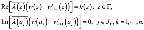
  has a unique solution. In fact, the boundary conditions (2.9), (2.10) can be rewritten in the form
 (2.11)
 (2.12)
Substituting the zero vector  into the position of
  on the right hand side of (2.11) and (2.12), by the hypothesis, the boundary value problem (2.11), (2.12) for analytic vectors has a unique solution
  and
and  Using the successive iterationwe can find a sequence
  of analytic vectors, which satisfies the boundary conditions
 (2.13)
 (2.14)
From (2.13) and (2.14), we have
 (2.15)
 (2.16)
In accordance with Theorem 2.1, we can conclude
 (2.17)
where  with
with , and
, and  Choosing a positive constant
 , such that
  it is not difficult to see that

and

for  where
where  is a positive integer. This shows that

Hence, there exists an analytic vector  such that
 (2.18)
Thus  is a solution of Problem
  with
with . From this we can derive that Problem
  with
with  i.e. Problem B for analytic vectors is solvable.
Next we prove the solvability of Problem B for the system (1.4).
Theorem 2.3 Let the nonlinear elliptic system (1.4) satisfy Condition C, and  in (1.6), (1.7), (1.11) be sufficiently small positive constants. Then Problem B for the complex system (1.4) is solvable.
Proof We consider the nonlinear elliptic complex system with the parameter :
:
 (2.19)
where  is any measurable vector in
  and
and  Applying Theorem 2.2, we see that Problem B for (2.19) with
  is solvable, and the solution
  can be expressed as
 (2.20)
where  is an analytic vector satisfying the boundary conditions
 (2.21)
 (2.22)
Suppose that when , Problem B for the system (2.19) has a unique solution. Then we shall prove that there exists a neighborhood of
  so that for every
  and any function
  Problem B for (2.19) is solvable. In fact, the complex system (2.19) can be written in the form
 (2.23)
Suppose that Problem B for (2.13) with  is solvable, by using the similar method as in the proof of Theorem 2.2, we can find a positive constant
 , so that for every
 , there exists a sequence
  of solutions satisfying
 (2.24)
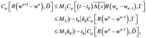
The difference of the above equations for  and
and  is as follows:
 (2.25)
From Condition C, we can derive that

and

Moreover,  satisfies the homogeneous boundary conditions
 (2.26)
 (2.27)
Similarly to Theorem 3.3, Chapter I, [1] , we have
 (2.28)
where  are positive constants. Provided
  is small enough, so that
  we can obtain
 (2.29)
for every  Thus
Thus

for  where
where  is a positive integer. This shows that
  as
as  Thus there exists a system of continuous functions
  in
in , such that

By Condition C, it follows that  is a solution of Problem B for the system (2.23), i.e. (2.19) for
 . It is easy to see that the positive constant
  is independent of
 . Hence Problem B for the system (2.19) with
  is solvable. Correspondingly we can derive that when
 , Problem B for (2.19) is solvable. Especially Problem B for (2.19) with
  and
and , namely Problem B for the system (1.4) has a solution.
3. Error Estimates of Approximate Solutions of the Discontinuous Riemann Hilbert Problem for Elliptic Systems of First Order Complex Equations
In this section, we shall introduce an error estimate of the above approximate solutions.
Theorem 3.1 Under the same conditions as in Theorem 2.3, let  be a solution of Problem B for the complex system (1.4) satisfying Condition C in
 , and
, and  be its approximation as stated in the proof of Theorem 2.3 with
  Then we have the following error estimate
 (3.1)
(3.1)
where  with
with  as in (2.28), and
  as in (1.6),(1.7), (1.11) and (1.16).
Proof From (1.4) and (2.24) with , we have
 (3.2)
(3.2)
It is clear that  satisfies the homogeneous boundary conditions
 (3.3)
(3.3)
Noting that  satisfy
 , and
, and

and then  is a solution of Problem
  for the complex equation
 (3.4)
(3.4)
hence we have
 (3.5)
(3.5)
in which
 (3.6)
(3.6)
where the non-negative constants  are as stated in (2.28), (1.5), (1.11) and (1.12). Moreover according to the proof of Theorem 2.3, we can derive
 (3.7)
(3.7)
From (3.6) and (3.7), it follows that

where  and
and  is the solution of Problem B for (2.24) with
  and
and  Finally, we obtain
 (3.8)
(3.8)
This shows that (3.1) holds. If the positive constant  is small enough, so that when
 is sufficiently large and
  is close to 1, then the right hand side becomes very small.
Note: The opinions expressed herein are those of the authors and do not necessarily represent those of the Uniformed Services University of the Health Sciences and the Department of Defense.
NOTES
*Deceased.
#I am very grateful for the guidance and help of Professor Guochun Wen, who served as my adviser for many years. 1 will always remember him because he inf1uenced me greatly.