1. Introduction
Stiffness is one of the most important performance indices of the PKMs, particularly for the use of high speed machining or heavy load assembling where high rigidity and dynamics are required. However, the complex geometry together with the changing rigidity of moving components throughout the whole workspace implies that to achieve a lightweight yet stiff design of PKMs is by no means an easy task. In the previous work dealing with stiffness analysis of PKMs, a great deal has been focused upon the formulation of the stiffness maps in the entire workspace by taking into account the limb rigidity [1] -[5] . By modeling a beam-like frame using FEA, a substructure-based modeling technique was proposed [6] [7] for quick stiffness estimation of a tripod PKM milling machine considering the rigidity of the machine frame.
The kinematic and static performances of the Tricept robot have been intensively investigated by Joshi and Tsai [8] by merely considering limb rigidity, in order to compare them with those of the 3-UPU parallel robot. Then a kinetostatic model for the Tricept is established by Zhang [9] based on lumped flexibilities theory, in order to account for joint and limb compliances.
2. Position Analysis
The schematic diagram of 3-PRS PKMs is showing in the Figure 1 below which is composed of moving platform, a fixed base and the three supporting limbs with identical configuration. Each limb connects the fixed base to the moving platform by prismatic, revolute and spherical joints in sequence and the prismatic joints are actuated by the linear actuator. The considered machine is a 3-DOF PKM a reference frame R is attached to the base and a body fixed frame R0 to the plate form with O and Oo located at the center of the equilateral triangle  and
and  as shown.
The Z and Z0 axes are normal to the planes of those triangles. The x axis is parallel to  and the
  axis is parallel to
 . Also an instantaneous reference frame Ro is set which its origin at point Oo and its three orthogonal axes remaining always parallel to those of R. Consequently the orientation matrix of R0 with respect to R can be obtained using three Euler angles
  in terms of precession nutation and body rotation according to the Z-X-Z convention.

Figure 1. Schematic diagram of 3-PRS PKM.
 ,
, 
where s ans c represents “sin” and “cos” respectively. The position vector , of p can be expressed as
 (1)
(1)
 ,
, 


The constraint imposed by the revolute joint restricts the translational motion of revolute joint in the limb
 ,
,  ,
,  ,
,
 (2)
(2)
3. Jacobian Analysis
The theory of reciprocal screw in an effective way to drive the Jacobian matrix of parallel manipulator; with  and
and  respectively denoting the vectors for the linear and angular velocities, the twist of the Mobil plat form can be defined as,
 .
.
A linear actuator drives each of prismatic joint. The connectivity of each limb is equals to five. Therefore the instantaneous twist  of the moving platform can be expressed as a linear combination of five instantaneous twist as follows.
 (3)
(3)
 ,
,  ,
,  ,
,  ,
, 
where  a unit vector along the jth joint axes of the ith limb. Those screw that are reciprocal to all the joint screws of the ith limb of the 3-PRS parallel kinematic manipulator form a 1-system. Hence one screw is reciprocal to all the joint screw of the limb can be identified. This reciprocal screw denoted as
  is zero pitch screw passing through the center of spherical joint and parallel to
 .
.
 (4)
(4)
By taking the inner product (orthogonal product) of both sides of the instantaneous twist Equation (3).

Writing the equation once for each limb produce 3 equations which can be written in matrix form.


Since this constraint wrench is reciprocal to all screw the right side equation of twist screw will be zero.
 (5)
(5)
Next we look the prismatic joint in each limb with actuator locked, the reciprocal screw for each limb form a two system. An additional basis screw which is reciprocal to the passive joints of the ith limb can be identified as zero pitch screw passing through the center of spherical joint. This reciprocal screw represent wrench of actuation and it’s normal to the pervious one system. That is

Take the orthogonal product of this reciprocal wrench for both side of the twist screw  this can be re write again


 (6)
(6)
And we can find  by orthogonal product of the right side of the above equation


Since this machine is not outer driving manipulator  will not be identity matrix. Then to fond the actuation Jacobian
 (7)
(7)

To find the overall Jacobian matrix by composing the actuation matrix in and constrained matrix on 

4. Stiffness Modeling
4.1. Stiffness Equations
Under the assumption that the platform and the machine frame are rigid, when the platform is subjected to the external wrench  on the reference point p, where
  and
and  are the external force and torque applied to the platform, the deformation of the limbs will causes the platform to experience a twist
  in terms of the translational and rotational deformations along/about the axes of frame.
Then, applying the virtual work principle to the platform gives
 (8)
(8)
where  and
and  represents the set of deflections and reaction force magnitude

This equation  can be re write
  Substitute
  from the above equation


Taking the transpose yields:

where  is the internal wrench vector of limbs, where
  and
and  are the generalized force of the PRS limbs and the PR limb related to the twist
 is a force which is parallel to the screw axis while the
  is parallel to the revolute axis.
Therefore the virtual work principle can be written


 (9)
(9)
 ,
,  and
and 
where .
.
Here  and
and  are known as the component stiffness matrix of actuation and constraints respectively the formulation of their element
 (10)
(10)
And the compliance model can be evaluated as .
.
4.2. Formulation of 
As shown in the Figure 2 above the limb model has to formulate . I group all the parts of a PRS limp in to four components: 1) the spherical joint; 2) the limp body which is the fixed lengths link; 3) R joint assembly; 4) the lead screw assembly. As well as analytically convenient, they are sub systems that must realistically be subjected independently to design improvements.
 is given in a diagonal matrix i.e.
  where
where  with
with  being the axial stiffness

Figure 2. A limb model for stiffness evaluation.
coefficient at  along the
  axis of the ith limb referring to the Figure 3.
  can be modeled by four serially connected springs each representing the stiffness of one of the four components such
 (11)
(11)
where ,
,  ,
,  and
and  are the axial stiff nesses coefficients of the lead screw assembly, the fixed length limb, S joint and R joint assembly respectively.
Note that , and
, and  are constant and can be evaluated using finite element analysis. (FEA) by the ANSYS workbench which is very convenient to analysis a solid model like PKM.
The  varies with the configuration and should be evaluated as in the local frame since the spherical actuation is parallel to w, the coefficient stuffiness is calculated as follows
 (12)
(12)
The values of Equation (12) can be substituted from Table 1 below.
 is the lead screw assembly the combination of serially connected springs such as
 (13)
(13)
where ,
,  and
and  are the stiffness coefficients of lead screw nut and support bearings respectively.
  is the lead screw which is the linear function of the limb length and can be defined as
 (14)
(14)
where  stands for cross sectional area of the lead screw and Yang’s modular respectively
  and
and  are the distance b/n the nut and the supporting bearing located at both ends.
To find the constrained coefficient of stiffness matrix we can find as the same fashion of finding the actuation coefficient matrix. Similarly


where  is the bending stiffness coefficient at the platform along the
  axis of the
  limb. Then
  can be evaluated by taking reciprocal sum of the bending stiffness coefficient of the fixed length limb, S joint and R joint assembly respectively.
 (15)
(15)
Again the  can be evaluated by the configuration and should be evaluated as in the local frame since the spherical parallel to the constraint is to u the coefficient stuffiness is calculated as follows

Table 1. The stiffness coefficient of the S joint.

Figure 3. Deformation with 1 KN force imposed at the spindle along y-axis.
 (16)
(16)
The value of the stiffness will be substitute from Table 1 and easy to compute the value of . The
. The  and
and  can be computed easy by FEA. Using the software ANSYS workbench by applying a 1 KN force on the spherical joint which is parallel to the
 .
.
4.3. Formulation of Overall Stiffness Matrix on Tool Tip
Formulation of overall stiffness matrix applied on the center of end-effectors is calculated on Equation (15) which is

To find the overall coefficient of stuffiness matrix on tool tip it needs to transform the Equation (10) in to tool tip by the transformation matrix
 (17)
(17)
If let  be imposed at the tool tip
  and
and  be the corresponding small deflection twist the overall stiffness matrix about point
  can easily be developed by replacing
  in Equation (10) with
  that is

where  is the distance from p to
 ,
,  denotes the screw matrix of
 , and
, and  denotes a unit matrix of order 3.


where .
.

 is the maximum radius of the cutting tool specified by the spindle head.

 (18)
(18)
In order to evaluate the rigidity of a system we define the rigidity along/about three orthogonal axis of the frame  by the diagonal corresponding element of C.
 ,
,  ,
,  ,
,  ,
,
 ,
,  ,
,  ,
, .
.
5. Stiffness Analysis
The stiffness of the 3-PRS PKM is evaluated in the decomposing the machine in to limbs and apply a force on the spherical joint to find the actuated and constraint coefficient of stuffiness. With the aid of finite element analysis and numerical evaluated both actuated and constraint stiffness of the limb assembly is evaluated. The overall stiffness of the manipulator on the center of the plate form will be calculated as in Equation (10) indicated. Since in real sense the force/moment is applied on the too tip of the machine, it needs transform the stiffness matrix gained in Equation (10) to the tool tip by the transform matrix Equation (16) it gives a stiffness coefficient matrix on tool tip as shown in the Equation (18). Then diagonal values in the stiffness matrix indicates the overall stiffness of the machine when force applied along x, y and z which explain in detail. In order to evaluate the rigidity of a system we define the rigidity along/about three orthogonal axis of the frame  by the diagonal corresponding element of C.
 ,
,  ,
,  ,
, .
.
Comparison with FEA Results
According to the above analysis, the detailed design was carried out and the stiffness of the virtual prototype was evaluated by ANSYS at four typical positions as shown from Figures 3-6 with 1 KN force is applied at the tool tip along x, y and z and moment about z axis respectively. I can get the deformation easily from the FEA and the stiffness can get by . It can been seen from Table 2 that the estimated results of the mathematical models developed have a good match with those obtained by the FEA in terms of magnitude and distribution as well.
The estimated linear stiffness along three orthogonal axis and the torsion stiffness about the w-axis of the  frame, it can be seen that the stiffness distribution are tri-symmetrical in nature and the
  and
and  are similar in magnitude.
6. Conclusions
The modeling methodology for the semi-analytical stiffness estimation of a 3-PRS parallel kinematic manipulator
Table 2. Results obtained by the semi-analytical method and by FEA.

Figure 4. Deformation with 1 KN force imposed at the spindle along x-axis.
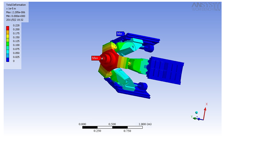
Figure 5. Deformation with 1 KN force imposed at the spindle along z-axis.

Figure 6. Deformation with 1 KN force imposed at the spindle moment about z.
has been systematically investigated by considering rigidity of the machine frame. The conclusions are drawn as follows:
1) The 6 × 6 Jacobian matrix consists of two sub matrices: one associated with the constraints imposed by the joints and the other associated with the actuation effects.
2) The stiffness model of machine as a whole can be generated mathematical model formulated in the conceptual design.
3) By the use of FEA with the tool of ANSYS work bench, I analyzed the machine stiffness and compared the FEA result with the semi-analytical analysis and the estimated stiffness results have a good match with those obtained by the FEA, thereby supporting the validity of this approach.