Bifurcations of Travelling Wave Solutions for the B(m,n) Equation ()
1. Introduction
Recently, Song and Shao [1] employed bifurcation method of dynamical systems to investigate bifurcation of solitary waves of the following generalized (2 + 1)-dimensional Boussinesq equation
 (1.1)
(1.1)
where  and
and  are arbitrary constants with
 . Chen and Zhang [2] obtained some double periodic and multiple soliton solutions of Equation (1.1) by using the generalized Jacobi elliptic function method. Further, Li [3] studied the generalized Boussinesq equation:
 (1.2)
(1.2)
by using bifurcation method. In this paper, we shall employ bifurcation method of dynamical systems [4] -[11] to investigate bifurcation of solitary waves of the following equation:
 (1.3)
(1.3)
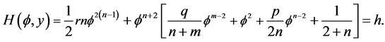
Numbers of solitary waves are given for each parameter condition. Under some parameter conditions, exact solitary wave solutions will be obtained. It is very important to consider the dynamical bifurcation behavior for the travelling wave solutions of (1.3). In this paper, we shall study all travelling wave solutions in the parameter space of this system. Let , where c is the wave speed. Then (1.3) becomes to
 (1.4)
(1.4)
where “'” is the derivative with respect to . Integrating Equation (1.4) twice, using the constants of integration to be zero we find
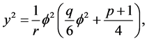
 (1.5)
(1.5)
where . Equation (1.5) is equivalent to the two-dimensional systems as follows
 (1.6)
(1.6)
with the first integral
 (1.7)
(1.7)
System (1.6) is a 5-parameter planar dynamical system depending on the parameter group . For different m, n and a fixed
 , we shall investigate the bifurcations of phase portraits of System (1.6) in the phase plane
  as the parameters
  are changed. Here we are considering a physical model where only bounded travelling waves are meaningful. So we only pay attention to the bounded solutions of System (1.6).
2. Bifurcations of Phase Portraits of (1.6)
In this section, we study all possible periodic annuluses defined by the vector fields of (1.6) when the parameters  are varied.
Let , Then, except on the straight lines
 , the system (1.6) has the same topological phase portraits as the following system
 (2.1)
(2.1)
Now, the straight lines  is an integral invariant straight line of (2.1).
Denote that
 (2.2)
(2.2)
For 
When ,
,
We have 
and which imply respectively the relations in the  -parameter plane


For 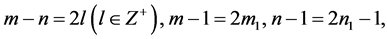 when
when ,
, We have
  and which imply respectively the relations in the
  parameter plane


For  when
when ,
, We have
 , which imply respectively the relations in the
  parameter plane

For  when
when ,
,  We have
  and
and which imply respectively the relations in the
  -parameter plane

Let  be the coefficient matrix of the linearized system of (2.1) at an equilibrium point
 . Then, we have

By the theory of planar dynamical systems, we know that for an equilibrium point of a planar integrable system, if  then the equilibrium point is a saddle point; if
  and
and  then it is a center point; if
  and
and ,.then it is a node; if
  and the index of the equilibrium point is
 then it is a cusp, otherwise, it is a high order equilibrium point.
For the function defined by (1.7), we denote that

We next use the above statements to consider the bifurcations of the phase portraits of (2.1). In the  parameter plane, the curves partition it into 4 regions for
  shown in Figure 1 (1-1), (1-2), (1-3), and (1-4), respectively.
1) The case , We use Figure 2, Figure 3, Figure 4, and Figure 5 to show the bifurcations of the phase portraits of (2.1).
2) The case . We consider the system
 (2.3)
(2.3)
with the first integral
 (2.4)
(2.4)
Figure 6 and Figure 7 show respectively the phase portraits of (2.3) for  and
and .
.
3. Exact Explicit Parametric Representations of Traveling Wave Solutions of (1.6)
In this section, we give some exact explicit parametric representations of periodic cusp wave solutions.
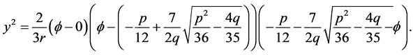
1). Suppose that , In this case, we have the phase portrait of (2.1) shown in Figure 2 (2-5). Corresponding to the orbit defined by
  to the equilibrium point
 , the arch curve has the algebraic equation
 (3.1)
(3.1)
Thus, by using the first equation of (1.6) and (3.1), we obtain the parametric representation of this arch as follows:
 (3.2)
(3.2)
where 
We will show in Section 4 that (3.10) gives rise to two periodic cusp wave solutions of peak type and valley type of (1.3).
2). Suppose that , In this case, we have the phase portrait of (2.1) shown in Figure 2 (2-4). corresponding to the orbit defined by
  to the equilibrium point
 , the arch curve has the algebraic equation
 (3.3)
(3.3)
Thus, by using the first equation of (1.6) and (3.3), we obtain the parametric representation of this arch as follows:

Figure 1. (1-1) m – n = 2l, n = 2n1; (1-2) m – n = 2l − 1, n = 2n1; (1-3) m – n = 2l, n = 2n1 + 1; (1-4) m – n = 2l-1, n = 2n1 + 1.

Figure 2. the phase portraits of (1.6) for m – n = 2l, n = 2n1,l, n1∈Z+. (2-1) r < 0, n1 = 2, (p, q) ∈ (A3); (2-2) r < 0, n1 ≥ 2, (p, q) ∈ (A3); (2-3) r > 0, n1 ≥ 2, (p, q) ∈ (A3); (2-4) r > 0, n1 = 1, (p, q) ∈ (A3); (2-5) r < 0, n1 = 2, (p, q) ∈ (A4); (2-6) r < 0, n1 ≥ 3, (p, q) ∈ (A3).

Figure 3. the phase portraits of (1.6) for m – n = 2l – 1, n = 2n1, l, n1∈Z+. (3-1) r < 0, n1 = 1, (p, q) ∈ (B1); (3-2) r < 0, n1 = 2, (p, q) ∈ (B1∪B2); (3-3) r > 0, n1 ≥ 2, (p, q) ∈ (B1) ∪(B2); (3-4) r > 0, n1 ≥ 2, (p, q) ∈ (B3); (3-5) r < 0, n1 = 2, (p, q) ∈ (B3); (3-6) r < 0, n1 ≥ 2, (p, q) ∈ (B1∪B2); (3-7) r < 0, n1 = 2, (p, q) ∈ (B4) ∪(B2); (3-8) r > 0, n1 ≥ 2, (p, q) ∈ (B4).
 (3.4)
(3.4)
We will show in Section 4 that (3.10) gives rise to a solitary wave solutions of peak type and valley type of (1.3).
3). Suppose that , In this case, we have the phase portrait of (2.1) shown in Figure 4 (4-5). corresponding to the orbit defined by
  to the equilibrium point
 , the arch curve has the algebraic equation
 (3.5)
(3.5)
where 
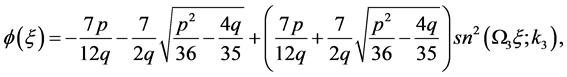
Thus, by using the first equation of (1.6) and (3.5), we obtain the parametric representation of this arch as follows:
 (3.6)
(3.6)
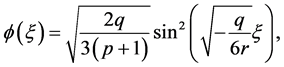
where  is the Jacobin elliptic functions with the modulo
 ,
,


We will show in Section 4 that (3.6) gives rise to a smooth compacton solution of (1.3).
4). Suppose that . In this case, we have the phase portrait of (2.1) shown in Figure 3 (3-1), corresponding to the orbit defined by
  to the equilibrium point
 , the arch curve has the algebraic equation
 (4-1)(4-2)(4-3)
  (4-4)(4-5)(4-6)
  (4-7)(4-8)(4-9)
 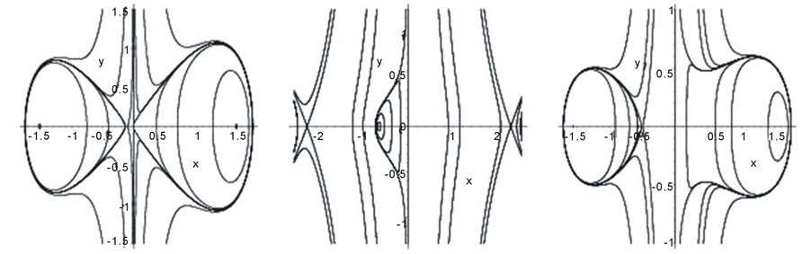 (4-10)(4-11)(4-12)
Figure 4. (4-1) r > 0, n1 = 1, (p, q) ∈ (C1); (4-2) r > 0, n1 ≥ 1, (p, q) ∈ (C2); (4-3) r > 0, n1 = 1, (p, q) ∈ (C2); (4-4) r > 0, n1 ≥ 2, (p, q) ∈ (C2); (4-5) r < 0, n1 = 1, (p, q) ∈ (C2); (4-6) r < 0, n1 ≥ 2, (p, q) ∈ (C2); (4-7) r > 0, n1 ≥ 2, (p, q) ∈ (C3); (4-8) r < 0, n1 = 1, (p, q) ∈ (C3); (4-9) r > 0, n1 = 1, (p, q) ∈ (C4); (4-10) r < 0, n1 = 1, (p, q) ∈ (C4); (4-11) r > 0, n1 ≥ 2, (p, q) ∈ (C4); (4-12) r < 0, n1 ≥ 2, (p, q) ∈ (C4).

Figure 5. the phase portraits of (1.6) for m – n = 2l – 1, n =2n1 + 1, l, n1∈Z+ (5-1) r > 0, n1 ≥ 2, (p, q) ∈ (D2); (5-2) r > 0, n1 = 1, (p, q) ∈ (D2); (5-3) r > 0, n1 ≥ 2, (p, q) ∈ (D3) ∪(D4); (5-4) r > 0, n1 = 1, (p, q) ∈ (D3) ∪(D4); (5-5) r < 0, n1 ≥ 2, (p, q) ∈(D3) ∪(D4); (5-6) r < 0, n1 = 1, (p, q) ∈(D3) ∪(D4); (5-7) r < 0, n1 ≥ 2, (p, q) ∈ (D2); (5-8) r < 0, n1 = 1, (p, q) ∈ (D2).
 (3.7)
(3.7)
Thus, by using the first equation of (1.6) and (3.7), we obtain the parametric representation of this arch as follows:
 (3.8)
(3.8)

Figure 6. The phase portraits of (1.6) for n = 2n1, n1∈Z+. (6-1) r < 0, n1 = 2, m1 ≥ n1, p < 0; (6-2) r < 0, n1 ≥ 2, m1 > n1, p < 0; (6-3) r > 0, m1 > n1, p < 0.

Figure 7. The phase portraits of (1.6) for n = 2n1 + 1, n1 ∈ Z+. (7-1) r > 0, n1 = 1, m1 ≥ n1, p > 0; (7-2) r < 0, n1 = 1, m1 > n1, p < 0; (7-3) r < 0, n1 ≥ 2, m1 > n1, p > 0, (7-4) r < 0, n1 ≥ 2, m1 > n1, p < 0.
We will show in Section 4 that (3.8) gives rise to a solitary wave solution of peak type or valley type of (1.3).
5). Suppose that  ,in this case, we have the phase portrait of (2.1) shown in Figure 5 (5-4). corresponding to the orbit defined by
  to the equilibrium point
 , the arch curve has the algebraic equation
 (3.9)
(3.9)
Thus, by using the first equation of (1.6) and (3.9), we obtain the parametric representation of this arch as follows:
 (3.10)
where  is the Jacobin elliptic functions with the modulo
  and
and


We will show in Section 4 that (3.10) gives rise to a smooth compacton solution of (1.3).
6). Suppose that , In this case, we have the phase portrait of (2.1) shown in Figure 5 (5-6), corresponding to the orbit defined by
  to the equilibrium point
 , the arch curve has the algebraic equation
 (3.11)
Thus, by using the first equation of (1.6) and (3.11), we obtain the parametric representation of this arch as follows:
 (3.12)
where 

we will show in Section 4 that (3.20) gives rise to a smooth compacton solution of (1.3)
7). Suppose  that. In this case, we have the phase portrait of (2.1) shown in Figure 3 (3-2) and (3-7), corresponding to the orbit defined by
  to the equilibrium point
 , the arch curve has the algebraic equation
 (3.13)
Thus, by using the first equation of (1.6) and (3.13), we obtain the parametric representation of this arch as follows:
 (3.14)
where 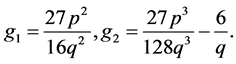 We will show in Section 4 that (3.14) gives rise to a smooth compacton solution of (1.3).
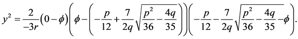
8). Suppose . In this case, we have the phase portrait of (2.1) shown in Figure 2 (2-1), corresponding to the orbit defined by
  to the equilibrium point
 , the arch curve has the algebraic equation
 (3.15)
Thus, by using the first equation of (1.6) and (3.15), we obtain the parametric representation of this arch as follows:
 (3.16)
where 

We will show in Section 4 that (3.16) gives rise to two periodic cusp wave solutions of peak type and valley type of (1.3).
9). Suppose . In this case, we have the phase portrait of (2.1) shown in Figure 4 (4-5), corresponding to the orbit defined by
  to the equilibrium point
 , the arch curve has the algebraic equation
 (3.17)
where  Thus, by using the first equation of (1.6) and (3.17)we obtain the parametric representation of this arch as follows:
 (3.18)
where  is the Jacobin elliptic functions with the modulo
  and
and


We will show in Section 4 that (3.6) gives rise to a smooth compacton solution of (1.3).
4. The Existence of Smooth and Non-Smooth Travelling Wave Solutions of (1.6)
In this section, we use the results of section 2 to discuss the existence of smooth and non-smooth solitary wave and periodic wave solutions. We first consider the existence of smooth solitary wave solution and periodic wave solutions.
Theorem 4.1
1). Suppose that : Then, corresponding to a branch of the curves
  defined by (1.7), equation (1.3) has a smooth solitary wave solution of peak type, corresponding to a branch of the curves
  defined by (1.7), equation (1.3) has a smooth family of periodic wave solutions (see Figure 4 (4-4)).
2). Suppose that : Then, corresponding to a branch of the curves
  defined by (1.7), equation (1.3) has a smooth solitary wave solution of peak type, corresponding to a branch of the curves
  defined by (1.7), equation (1.3) has a smooth family of periodic wave solutions (see Figure 4 (4-3)).
3). Suppose that , Then, corresponding to a branch of the curves
  defined by (1.7), equation (1.3) has a smooth solitary wave solution of peak type, corresponding to a branch of the curves
  defined by (1.7), equation (1.3) has a smooth family of periodic wave solutions (see Figure 4 (4-12)).
4). Suppose that , Then, corresponding to a branch of the curves
  defined by (1.7), equation (1.3) has a smooth solitary wave solution of valley type, corresponding to a branch of the curves
  defined by (1.7), equation (1.3) has a smooth family of periodic wave solutions (see Figure 4 (4-3)).
5). Suppose that , Then, corresponding to a branch of the curves
  defined by (1.7), equation (1.3) has a smooth solitary wave solution of peak type, corresponding to a branch of the curves
  defined by (1.7), equation (1.3) has a smooth family of periodic wave solutions (see Figure 2 (2-3)).
6). Suppose that , Then, corresponding to a branch of the curves
  defined by (1.7), equation (1.3) has a smooth solitary wave solution of peak type, corresponding to a branch of the curves
  defined by (1.7), equation (1.3) has a smooth family of periodic wave solutions (see Figure 2 (2-3)).
7). Suppose that , Then, corresponding to a branch of the curves
  defined by (1.7), equation (1.3) has a smooth solitary wave solution of valley type, corresponding to a branch of the curves
  defined by (1.7), equation (1.3) has a smooth family of periodic wave solutions (see Figure 2 (2-3)).
8). Suppose that , Then, corresponding to a branch of the curves
  defined by (1.7), equation (1.3) has a smooth family of periodic wave solutions (see
Figure 3 (3-5)).
9). Suppose that: , Then, corresponding to a branch of the curves
  defined by (1.7), equation (1.3) has a smooth solitary wave solution of valley type, corresponding to a branch of the curves
  defined by (1.7), equation (1.3) has a smooth family of periodic wave solutions (see Figure 3 (3-4)).
10). Suppose that , Then, corresponding to a branch of the curves
  defined by (1.7), equation (1.3) has a smooth solitary wave solution of valley type, corresponding to a branch of the curves
  defined by (1.7), equation (1.3) has a smooth family of periodic wave solutions (see Figure 2 (2-4)).
11). Suppose that : Then, corresponding to a branch of the curves
  defined by (1.7), equation (1.3) has a smooth solitary wave solution of valley type, corresponding to a branch of the curves
  defined by (1.7), equation (1.3) has a smooth family of periodic wave solutions (see Figure 3 (3-1)).
We shall describe what types of non-smooth solitary wave and periodic wave solutions can appear for our system (1.6) which correspond to some orbits of (2.1) near the straight line . To discuss the existence of cusp waves, we need to use the following lemmarelating to the singular straight line.
Lemma 4.2 The boundary curves of a periodic annulus are the limit curves of closed orbits inside the annulus; If these boundary curves contain a segment of the singular straight line  of (1.4), then along this segment and near this segment, in very short time interval
  jumps rapidly.
Base on Lemma 4.2, Figure 2, and Figure 3, we have the following result.
Theorem 4.3
1). Suppose that 
a). For  corresponding to the arch curve
  defined by (1.7), equation (1.3) has two periodic cusp wave solutions; corresponding to two branches of the curves
  defined by (1.7), equation (1.3) has two families of periodic wave solutions. When h varies from
  to 0, these periodic travelling waves will gradually lose their smoothness, and evolve from smooth periodic travelling waves to periodic cusp travelling waves, finally approach a periodic cusp wave of valley type and a periodic cusp wave of peak type defined by
  of (1.7) (see Figure 2 (2-5)).
b). For  corresponding to the arch curve
  defined by (1.7), equation (1.3) has two periodic cusp wave solutions; corresponding to two branches of the curves
defined by (1.7), equation (1.3) has two families of periodic wave solutions. When h varies from  to 0, these periodic travelling waves will gradually lose their smoothness, and evolve from smooth periodic travelling waves to periodic cusp travelling waves, finally approach a periodic cusp wave of valley type and a periodic cusp wave of peak type defined by
  of (1.7) (see Figure 2 (2-1)).
2). Suppose that 
c). For  corresponding to the arch curve
  defined by (1.7), equation (1.3) has two periodic cusp wave solutions; corresponding to two branches of the curves
  defined by (1.7), equation (1.3) has two families of periodic wave solutions. When h varies from 0 to
 , these periodic travelling waves will gradually lose their smoothness, and evolve from smooth periodic travelling waves to periodic cusp travelling waves, finally approach a periodic cusp wave of valley type and a periodic cusp wave of peak type defined by
  of (1.7) (see Figure 3 (3-7)).
d). For  corresponding to the arch curve
  defined by (1.7), equation (1.3) has two periodic cusp wave solutions; corresponding to two branches of the curves
  defined by (1.7), equation (1.3) has two families of periodic wave solutions. When h varies from 0 to
 , these periodic travelling waves will gradually lose their smoothness, and evolve from smooth periodic travelling waves to periodic cusp travelling waves, finally approach a periodic cusp wave of valley type and a periodic cusp wave of peak type defined by
  of (1.7) (see Figure 3 (3-5)).
d). For  corresponding to the arch curve
  defined by (1.7), equation (1.3) has two periodic cusp wave solutions; corresponding to two branches of the curves
  defined by (1.7), equation (1.3) has two families of periodic wave solutions. When h varies from 0 to
 , these periodic travelling waves will gradually lose their smoothness, and evolve from smooth periodic travelling waves to periodic cusp travelling waves, finally approach a periodic cusp wave of valley type and a periodic cusp wave of peak type defined by
  of (1.7) (see Figure 3 (3-3)).
We can easily see that there exist two families of closed orbits of (1.3) in Figure 2 (2-6), Figure 3 (3-6) and in Figure 6 (6-2). There is one family of closed orbits in Figure 3 (3-3), (3-8), Figure 4 (4-2), (4-5) - (4-7), (4-9), (4-11) and in Figure 5 (5-3), (5-5) - (5-7) and in Figure 7 (7-3), (7-4). In all the above cases there exists at least one family of closed orbits (1.3) for which as whichh from  to 0, where
  is the abscissa of the center, the closed orbit will expand outwards to approach the straight line
  and
and  will approach to
 . As a result, we have the following conclusions.
Theorem 4.4
1). Suppose that 
a). If ; then when
  in (1.7), Equation (1.3) has a family of uncountably infinite many periodic traveling wave solutions; where
  varies from
  to 0, these periodic traveling wave solutions will gradually lose their smoothness, and evolve from smooth periodic traveling waves to periodic cusp traveling waves (see Figure 4 (4-2)).
b). If ; then when
  in (1.7), Equation (1.3) has a family of uncountably infinite many periodic traveling wave solutions; when
  varies from 0 to
 , these periodic traveling wave solutions will gradually lose their smoothness, and evolve from smooth periodic traveling waves to periodic cusp traveling waves (see Figure 4 (4-7)).
c). If ; then when
  in (1.7), Equation (1.3) has a family of uncountably infinite many periodic traveling wave solutions; when
  varies from 0 to
 , these periodic traveling wave solutions will gradually lose their smoothness, and evolve from smooth periodic traveling waves to periodic cusp traveling waves (see Figure 4 (4-6)).
d). If ; then when
  in (1.7), Equation (1.3) has a family of uncountably infinite many periodic traveling wave solutions; when
  varies from
  to 0, these periodic traveling wave solutions will gradually lose their smoothness, and evolve from smooth periodic traveling waves to periodic cusp traveling waves (see Figure 4 (4-11)).
e). If ; then when
  in (1.7), Equation (1.3) has a family of uncountably infinite many periodic traveling wave solutions; when
  varies from 0 to
 , these periodic traveling wave solutions will gradually lose their smoothness, and evolve from smooth periodic traveling waves to periodic cusp traveling waves (see Figure 4 (4-5)).
f). If ; then when
  in (1.7), Equation (1.3) has a family of uncountably infinite many periodic traveling wave solutions; when
  varies from 0 to
 , these periodic traveling wave solutions will gradually lose their smoothness, and evolve from smooth periodic traveling waves to periodic cusp traveling waves (see Figure 4 (4-9)).
2). Suppose that ,then when  in (1.7), Equation (1.3) has two family of uncountably infinite many periodic traveling wave solutions; when
  varies from 0 to
 , these periodic traveling wave solutions will gradually lose their smoothness, and evolve from smooth periodic traveling waves to periodic cusp traveling waves (see Figure 2 (2-6)).Parallelling to Figure 2 (2-6), we can see the periodic travelling wave solutions implied in Figure 3 (3-6) and Figure 6 (6-2) have the same characters.
3). Suppose that 
g). If ; then when
  in (1.7), Equation (1.3) has a family of uncountably infinite many periodic traveling wave solutions; when
  varies from 0 to
 , these periodic traveling wave solutions will gradually lose their smoothness, and evolve from smooth periodic traveling waves to periodic cusp traveling waves (see Figure 5 (5-6)).
h). If ; then when
  in (1.7), Equation (1.3) has a family of uncountably infinite many periodic traveling wave solutions; when
  varies from 0 to
 , these periodic traveling wave solutions will gradually lose their smoothness, and evolve from smooth periodic traveling waves to periodic cusp traveling waves (see Figure 5 (5-7)).
i). If , then when
  in (1.7), Equation (1.3) has a family of uncountably infinite many periodic traveling wave solutions; when
  varies from
  to 0, these periodic traveling wave solutions will gradually lose their smoothness, and evolve from smooth periodic traveling waves to periodic cusp traveling waves (see Figure 5 (5-3)).
j). If , then when
  in (1.7), Equation (1.3) has a family of uncountably infinite many periodic traveling wave solutions; when
  varies from 0 to
 , these periodic traveling wave solutions will gradually lose their smoothness, and evolve from smooth periodic traveling waves to periodic cusp traveling waves (see Figure 5 (5-5)).
4). Suppose that 
k). If , then when
  in (1.7), Equation (1.3) has a family of uncountably infinite many periodic traveling wave solutions; when
  varies from
  to 0, these periodic traveling wave solutions will gradually lose their smoothness, and evolve from smooth periodic traveling waves to periodic cusp traveling waves (see Figure 5 (5-5)).
Equation (1.3) has one family of uncountably infinite many periodic traveling wave solutions; when  varies from 0 to
 , these periodic travelling wave solutions will gradually lose their smoothness, and evolve from smooth periodic travelling waves to periodic cusp travelling waves (see Figure 7 (7-4)).
Acknowledgements
This work is supported by t NNSF of China (11061010, 11161013). The authors are grateful for this financial support.
NOTES
*Corresponding author.