1. Introduction
The idea of canalization was initiated from Waddington, C. H. [2]. When comparing the class of canalyzing functions to other classes of functions with respect to their evolutionary plausibility as emergent control rules in genetic regulatory systems, it is informative to know the number of canalyzing functions with a given number of input variables [1]. However, the Boolean network modeling paradigm is rather restrictive, with its limit to two possible functional levels, ON and OFF, for genes, proteins, etc. Many discrete models of biological networks therefore allow variables to take on multiple states. Common used discrete multi-state model types are socalled logical models [3], Petri nets [4], and agentbased models [5].
In this paper, we generalize the concept of Boolean canalyzing rules to the multi-state case. By generalizing the results in [1], we provide formulas for the cardinalities of various subsets of canalyzing functions. We also obtain the asymptotes of these cardinalities as either  or
or . We obtain a combinatorial identity by equating our result to the formula in [1].
2. Preliminaries
In this section we introduce the definition of a canalyzing function.
Let  and
and  .
.
A function is canalyzing if there is a variable  and an element
  so that the value of the function is fixed once variable
  is fixed at
 . More precisely, we have the following definitions.
Definition 2.1
1) The function  is
is  canalyzing if
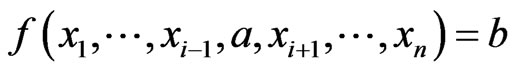 , for all
  .
.
2) The function  is
is  canalyzing if there exists
  such that
  , for all
  .
.
3) The function  is
is  canalyzing if there exists
  such that
 , for all
  .
.
4) The function  is
is  canalyzing if there exists
  such that
  , for all
  .
.
5) The function  is
is  canalyzing if there exist
  such that
  , for all
  .
.
6) The function  is
is  canalyzing if there exist
 ,
,  such that
  , for all
  .
.
7) The function  is
is  canalyzing if there exist
  such that
  , for all
  .
.
8) The function is  is
is  canalyzing if there exist
  such that
  , for all
  .
.
By abuse of notation, we also use  to stand for the set of all the
  canalyzing functions,
  will stand for the set of all the
  canalyzing functions and etc. We use
  to stand for the empty set.
By the definitions, we immediately have the following propositions.
Proposition 2.2 If , then
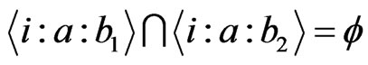 .
.
Proposition 2.3 If  and
and , then
  .
.
By the definitions, we have

For any set , we use
  to stand for its cardinality.
We use  to stand for the binomial coefficients. As usual,
  should be explained as zero once
 .
.
Obviously, for the above notations, the cardinality are same for different values of  and
and . In other wordswe have
 ,
,
 ,
,  and etc.
3. Enumeration
Theorem 3.1 Given , the number of
 canalyzing functions is
 . In other wordswe have
 .
.
Proof: A function in the set  is uniquely determined by its value on inputs
  with
with  . There are
  such inputs, and the function can take
  different values. Thus
  . □
. □
Because , by Proposition 2.2we get Theorem 3.2 The number of all the
  canalyzing function is

Lemma 3.3 We have  for any
 .
.
Proof: A function in the set  is uni quely determined by it values on inputs
  with
with . There are
  such inputs. □
Theorem 3.4 Given  and
and , the number of
  canalyzing functions is
 . In other words, we have
 .
.
Proof: By Inclusion and Exclusion Principle, we have

Similar to Lemma 3.3, we have Lemma 3.5 If , then
 .
.
Based on this lemma, we can get the following result.
Theorem 3.6 We have

Proof: By Inclusion and Exclusion Principle, we have

From the above theorem, we can get the following result.
Theorem 3.7 We have
Proof: Because , by Theorem 3.6, we just need to show
 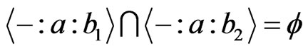 if
if  . Suppose
 , then there exist
  and
and  such that
 since
since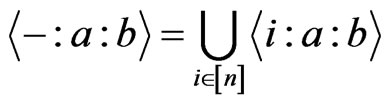 .
.
If , we get a contradiction by Proposition 2.2. If
 , we get a contradiction by Proposition 2.3 since
  and
and . □
. □
Now, we are going to find the formula for the number of all the canalyzing functions with given canalyzed value . In other words, the formula of
 .
.
Let  for any
 . By Inclusion and Exclusion Principle, we have

where

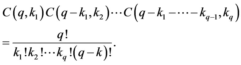
In order to evaluate , we write all the members in
  as the following
  matrix.

For any  with
with , we will choose
  elements from the above matrix to form
 .
.
Suppose  of its elements are from the first row (there are
  ways to do so). Let these
  elements be
 .
.
Suppose  of its elements are from the second row (there are
  ways to do so). Let these
  elements be
 .
.

Suppose  of its elements are from the last row (there are
  ways to do so). Let these
  elements be
 .
.
 .
.
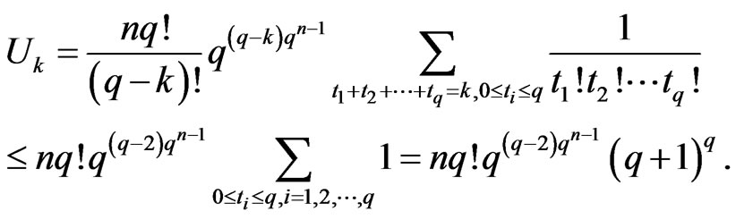
Similar to Lemma 3.3, we have Lemma 3.8 Let  be the subset of
  as mentioned above, then
 .
.
Hence,

We get Theorem 3.9 For any , we have

In order to evaluate , we need two more lemmas. Their proofs are similar to that of Lemma 3.3 and we omit them.
Lemma 3.10 If  and
and  , then
 .
.
Lemma 3.11 If  are
are  distinct elements of
 ,
,  . Then,

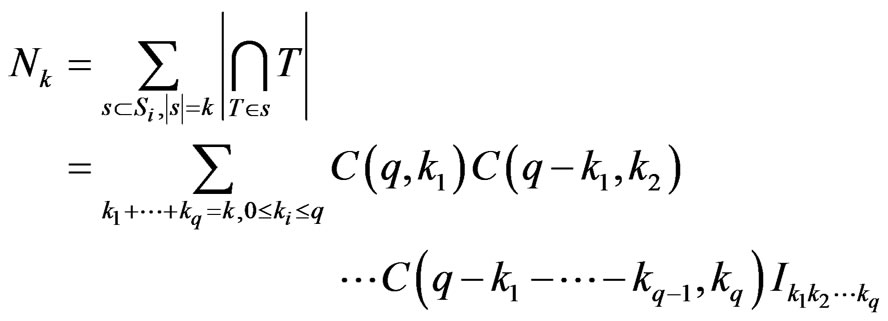
Now, we are ready to find the cardinality of .
.
Theorem 3.12 We have

Proof: First, we have .
.
Let , we get
 . Where

In order to evaluate , we write all the elements in
  as the following
  matrix.

For any  with
with , we will choose
  elements from the above matrix to form
 .
.
Suppose  of it elements are from the first row (There are
  ways to do so). Let these
  elements be
 .
.
Suppose  of its elements are from the second row, we must choose these elements from different columns, otherwise the intersection will be
  by Proposition 2.2 (There are
  ways to do so). Let these
  elements be

Suppose  of its elements are from the last row (There are
  ways to do so). Let these
  elements be
 .
.
where . We have
where

By Lemma 3.11, we know

This number is zero if .
.
A straightforward computing shows that
Hence, we get

□
Now we begin to evaluate .
.
Theorem 3.13 We have

where

and

Proof: Let

We have

and , where

We write all the  elements of S as the following
  matrices.

We combine all the above  to form a
  matrix
  whose first
  rows are
 , the second
  rows are
  the last
  rows are
 . In other words, we have

We are going to choose  elements from
  to form the intersection. In order to get a possible non empty intersection, we know all these
  elements must come from either the same
  (for some fixed
 ) or all of them from the same column of
  by Proposition 2.3.
Each  is in fact the transpose of
  and each column of
  is all the elements of
  (As sets, they are equal). Hence, a typical intersection is either the one in Theorem 3.9 or the one in Theorem 3.12. But these two cases are not disjoint.
Suppose we choose  elements from
 .
.
If there exist  such that
 , then
 . This implies the intersection looks like the one in Lemma 3.11 and
 .
.
If , then the intersection looks like the one in Lemma 3.8 and
 .
.
The above two cases are disjoint now. By Lemma 3.11 and Lemma 3.8, we get

where (Note: there are  matrices
  and
and  columns of
 )
)

Hence,
 □
□
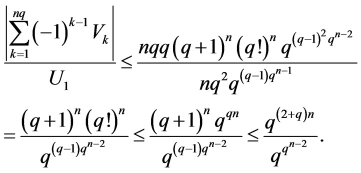
In the following, we will reduce the formula

when  and compare it with the one in [1]. We have

where

A simple calculation shows that

and
 since the condition of the sum is not satisfied.

Note,  is the number of solutions of the equation
 .
.
When ,
,

Note,  is the number of solutions of the equation
 ,
,  with exactly
  components equal to 2.
hence, when ,
,

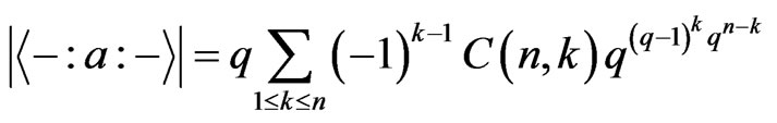
When , one can obtain (without calculator) the sequence 4, 14, 120, 3514. These results are consistent with those in [1]. By [1], the cardinality of
  should be

So, we obtain the following combinatorial identity(for any positive integer ).
).

The left sum should be explained as 0 if . As usual,
  is 0 if
 .
.
From Theorem 3.1, we know since
since , we obtain
 .
.
In order to get an intuitive idea about the magnitude of all the cardinality numbers, We will find their asymptote as  or
or .
.
We have the following notation Definition 3.14 We call  if
if 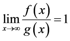 .
.
Now, we can list all the cardinalities asymptotically.
Theorem 3.15 If  and
and , then

Proof:
The first two rows are Theorem 3.1 and Theorem 3.2.
We will give a proof of the last row, the others are similar and easier.

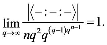
When , we have
Hence,
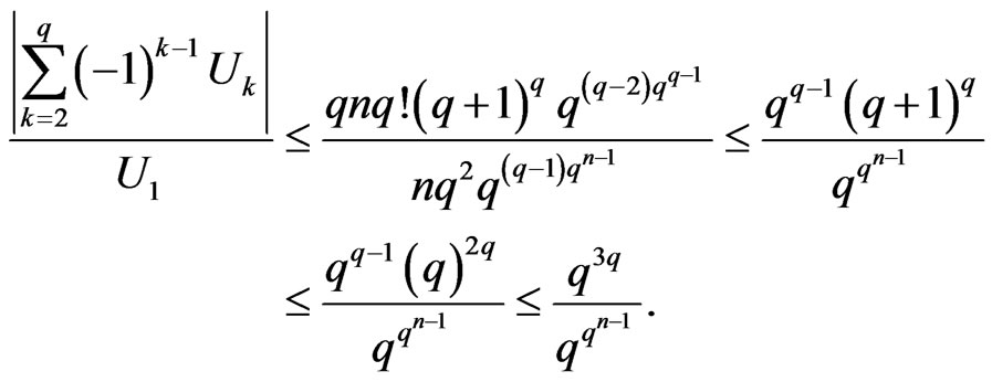
So, .
.
 since the condition of the sum is not satisfied.
When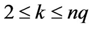 , we have

Note, . Hence,

We obtain
Hence,

In summary, we obtain

In other words,

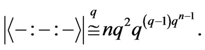
From the above proof, it is also clear that we have
In other words,
□
When , the first equation of the last row in the above theorem has been obtained in [1].
4. Conclusion
In this paper, we generalized the definition of Boolean canalyzing functions to the functions of multi-state case. Using Inclusion and Exclusion Principle, we get formulas for the cardinality all such functions and the cardinalities of its various subsets. When , we derive an interesting combinatorial identity by equating our formula to the one in [1]. Finally, for a better understanding to the magnitudes, we provide all the asymptotes of these cardinalities as either
  or
or .
.
5. Acknowledgements
This work was initiated when the first and the third authors visited Virginia Bioinformatics Institute at Virginia Tech in June 2010. We thank Alan Veliz-Cuba and Franzeska Hinkelmann for many useful discussions. The first and the third authors thank Professor Reinhard Laubenbacher for his hospitality and for introducing them to Discrete Dynamical Systems. The third author was supported in part by a Research Initiation Program (RIP) award at Winston-Salem State University.
We greatly appreciate an anonymous reader. Because of his insightful comments, in this paper, the proofs for many lemmas are simplified, the results are more general (On any finite set instead of finite field).
NOTES
*Corresponding author.