Electrical Impedance Tomography Image Reconstruction Using Iterative Lavrentiev and L-Curve-Based Regularization Algorithm ()
1. Introduction
Electrical impedance tomography (EIT) is an imaging technique which determines the electrical conductivity and permittivity distribution within a medium using electrical measurement from a series of electrodes on its surface [1–3]. Electrodes are brought into contact with the surface of the object being imaged. A set of voltage (or current) are applied and the corresponding currents (or voltage) are measured [4]. These voltages and currents are then used to estimate the electrical properties of the object using an image reconstruction algorithm [5]. The relatively poor spatial resolution of the reconstructed images in EIT is often quoted as its major disadvantages, compared with already established scanners with good resolution. In this respect, it must be clarified that the motivation of EIT is somewhat different from that of the conventional imaging techniques. Despite its limited resolution, its task is to provide a reliable, real-time, portable and cost efficient imaging tool. Depending on the particular application and the resolution specifications, EIT can sometimes provide an optimum cost-effective imaging solution. Example application areas include geophysical inversion [6], industrial process monitoring [7], and medical diagnosis [8].
However, the process of property estimation in EIT is a highly nonlinear, ill-conditioned, and ill-posed problem. The sensitivity matrix, which relates interior admittivity perturbations to perturbations in the boundary data, is heavily ill-conditioned with respect to inversion. So, it requires special treatment in the form of regularization or a truncation of a singular value expansion [9]. When approaching an ill-posed problem, instead of attempting to solve the original problem one often opts to solve a similar one which is less demanding. Therefore, effective EIT image reconstruction algorithms are required.
Some papers on image reconstruction algorithms have been published [10–14], but little work on EIT image reconstruction is published. The first proposed EIT reconstruction algorithm is the equipotential back-projection [15]. This technique reconstructs images by projecting the change in measurements at each electrode pair across the equipotential region for that current injection pattern, multiplied by an image filter. However, unlike the X-ray used in CAT scanning or general inverse scattering problems [16]. Currents in EIT do not move in a line, but cover the region from the current source to drain. A bias is thus introduced into the image since the equipotential region is an approximation to the region producing the measurement change at each electrode. A finite element-based reconstruction algorithm was proposed in [7], but limited scalar/vectors can be reconstructed with this algorithm. A reconstruction algorithm for breast tumor imaging based on linearization approach was proposed in [8], but the number of independent conductivity regions that can be calculated is too small. In [17] it was assumed that the resistivity distribution could be well approximated as a linear combination of some preselected basis functions. Prior information on the structures and conductivities were used for the construction of these basis functions. The disadvantage of this method is that one may obtain misleading results when prior information is incompatible.
In this paper, we propose an iterative Lavrentiev regularization-based algorithm to reconstruct EIT images using knowledge of the noise variance of the measurements and the covariance of the conductivity distribution. As the regularization parameter should be carefully chosen, an L-curve-based optimization algorithm is applied. Numerical analysis and simulation results are provided. The remaining sections are organized as follows. Section 2 forms the problem of EIT image reconstruction and outlines the motivations of this paper. Section 3 details the iterative Lavrentiev regularization-based EIT reconstruction algorithm, followed by the simulation examples in Section 4. Finally, Section 5 concludes the whole paper.
2. Electrical Impedance Tomography (EIT)
Taking EIT imaging in medical applications as an example [18,19], different tissues of the body are shown to have different electrical characteristics. Most tissues can be considered isotropic with the exception of muscles and brain tissue which are anisotropic. It is usually assumed to be homogenous and isotropic, where the constitute parameters such as the conductivity and permittivity are independent of position and direction. Therefore, the underlying relationships that govern the interaction between EIT electricity and magnetism are the Maxwell’s equations. The medium ( ) is modeled as a closed and bounded subset of three-dimensional space with smooth boundary (
 ) and uniform conductivity (
 ). The electric field (
 ) enclosed in
  is expressed in terms of the scalar potential
 , (1)
, (1)
where
 (2)
(2)
is the vector differential operator, and  is the potential in the medium. The current (
 ) is given by the multiplication of the conductivity. The electric field can then be computed as
 . (3)
. (3)
As there are no interior current sources, EIT simulation in the medium can be described in terms of a scalar voltage potential satisfying Kirchoff’s voltage law
 . (4)
. (4)
The boundary current density ( ) can then be represented by
 . (5)
. (5)
According to this relationship, the problem of determining the potential inside the medium from boundary measurements can then be carried out [20].
3. Iterative Lavrentiev Regularization and L-Curve-Based EIT Image Reconstruction
To apply regularization-based image reconstruction methods, EIT problems can be formulated as a system of linear equations [21]
 (6)
(6)
where  is the nodal potential distribution,
  is the potential values on the boundary electrodes,
  ,
,  and
and  are the local matrices. This equation can be represented by
 (7)
(7)
where  is the error in the data with
  and
and . One standard approach used to solve linear estimation problems is the least square estimation, but this estimate is unsatisfactory because the calculated independent conductivity region is too small.
The inverse of the A cannot be directly computed because the singular values will grow without bound. This will amplify the noise components in the solution associated with the numerical null space of . That is to say, small measurement perturbations
  may produce large variations in
  such that the 3-norm residual error
  is unbounded. Therefore, the matrix
  is poor conditioned because EIT makes current injection and measurement on the medium surface including higher current densities near the surface where conductivity contrasts will result in more signal than for contrasts in the center. This problem can be resolved by regularization [22]. That is, assume
  is an invertible and real-valued matrix, it can then be decomposed by singular value decomposition (SVD)
 (8)
(8)
Correspondingly, Equation (7) can be expressed by
 (9)
(9)

Figure 1. Tikhonov-based regularization filter  at different

Figure 2. The norm of the regularization solution errors as a function of the regularization parameter of 
As instability may arises due to division by small singular values, to overcome this problem we apply an iterative Lavrentiev-based regularization algorithm.
Lavrentiev regularization replaces Equation (7) by [23]
 , (10)
where  is the regularization parameter. Correspondingly, the iterative Lavrentiev regularization is
 (11)
(11)
This equation can be changed into
 (12)
(12)
Suppose the solution of the Equation (7) is 
 (13)
(13)
where  is the normalized function with
 . Note that
  refers to the smoothness source conditions. Considering the function
 (14)
(14)
when , it arrives its maximum
 (15)
(15)
Hence, we have
 (16)
(16)
where  is a constant parameter for the specific
 . Therefore, this algorithm is converged with a convergence rate of
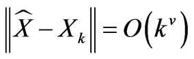 (17)
(17)
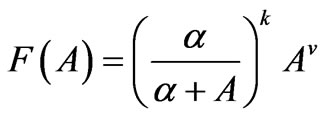
In fact, the Lavrentiev regularization just uses the filter function
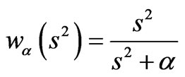 (18)
(18)
with a regularization parameter of , as shown in Figure 1. In conventional regularization-based reconstructed algorithms, the regularization parameter is often heuristically selected; however, it determines the cut-off of the filter, as shown in Figure 2. Further analysis results show that when the regularization parameter is very small, filtering of the noise will be inadequate and
  will be highly oscillatory. In contrast, when the regularization parameter is too large, the reconstructed image will be overly smooth. Therefore, some effective algorithms should be developed to optimize the regularization parameter. To reach this aim, we apply an L-curve [24]- based optimization algorithm.
L-curve is a parametric plot of the squared norm of the regularized solution against the squared norm of the regularized residual for a range of values of regularization parameter. The L-curve criterion for regularization parameter selection is to pick the parameter value corresponding to the “corner” of this curve. Let  denote the regularized solution and let
  denote the regularized residual. Define
 (19)
(19)
 (20)
(20)
We can then select the value of  that maximizes the curvature function
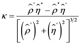 , (21)
where  and
and  are represented, respectively, by
 , (22)
 , (23)
The ,
,  ,
,  and
and  denote the first and second derivatives of
 ,
,  with respect to
 . As shown in Figure 3, the L-curve has two characteristic parts: the more horizontal where the solution is dominated by the regularization errors, the vertical part where the solution is dominated by the right-hand errors. The solutions are overand under-smoothed, respectively. The corner of the L-curve corresponds to a good balance between minimization of the sizes, and the corresponding regularization parameter
  is a good one. In this way, an optimum regularization parameter
  can be optimization determined.

Figure 5. Iterative Lavrentiev reconstructed image with 
4. Simulation Examples
In many industrial process and biomedical EIT applications, it is often the case that one knows in advance what materials (tissues) are included within the measurement domain. As mixtures of materials are known to have intermediate conductivities, this effectively restricts the admissible solutions, i.e., the pixels of the reconstructed images, to lie within a set of known values. In this sense, the bound-constrained (with bounds on the values of the admittivity distribution) is to locate the detected inhomogeneities.
As an example, one can allow that the admittivity distribution to be reconstructed is mainly homogenous with an unknown number of shaped inclusions. In EIT applications, the current with a frequency of 10-100kHz is widely used. These patterns are similar to those appearing in Figure 4, which shows the simulated admittivity distribution with the three inhomogeneity patterns. Although the geometry (shape and dimension) of these patterns is assumed to be known a priori, their number, admittivity values and exact location are to be recovered from the
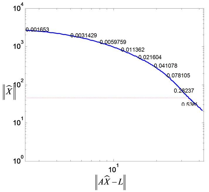
Figure 6. Regularization selection with L-curve-based optimization algorithm

Figure 7. Iterative Lavrentiev reconstructed image with L-curve optimized regularization parameter
image reconstruction. For the reconstructions, simulated measurements contaminated with 2% Gaussian noise have been assumed. Regularization parameter  is often used in conventional regularizationbased reconstruction methods, e.g., [25], but from Figure 5 we notice that it fails to capture the boundary shape and interior gap of the inhomogeneities. To get around this disadvantage, the regularization parameter is optimized with the L-curve algorithm, as shown in Figure 6. Correspondingly, Figure 7 gives the reconstructed image using the optimized regularization parameter (here is
 ). Comparing the two images, the enhancement is obvious. This result comes in support of the fact that this method is robust to noise.
5. Conclusions
EIT is a technique used to create images of the electrical properties in the interior of a medium from measurements on its boundary, which is particularly important for medical and industrial applications [26,27]. Usually a set of voltage or current measurements is acquired from the boundaries of a conductive volume. In this paper, we presented an iterative Lavrentiev regularization and Lcurve-based algorithm to reconstruct EIT images using knowledge of the noise variance of the measurements and the covariance of the conductivity distribution. The regularization parameter should be carefully selected, but it is often heuristically selected in conventional regularization-based reconstruction algorithms. So, an L-curvebased optimization algorithm is applied to choose the Lavrentiev regularization parameter. The method is validated with numerical analysis and simulation results. Further research efforts are planned to focus on experimental investigations [28,29] and other computational electromagnetic-based algorithms [30].
NOTES