Some Results for Exact Support Recovery of Block Joint Sparse Matrix via Block Multiple Measurement Vectors Algorithm

Abstract

Block multiple measurement vectors (BMMV) is a reconstruction algorithm that can be used to recover the support of block K-joint sparse matrix X from Y = ΨX + V. In this paper, we propose a sufficient condition for accurate support recovery of the block K-joint sparse matrix via the BMMV algorithm in the noisy case. Furthermore, we show the optimality of the condition we proposed in the absence of noise when the problem reduces to single measurement vector case.

Share and Cite:

Pan, Y. and Zhang, P. (2023) Some Results for Exact Support Recovery of Block Joint Sparse Matrix via Block Multiple Measurement Vectors Algorithm. Journal of Applied Mathematics and Physics, 11, 1098-1112. doi: 10.4236/jamp.2023.114072.

1. Introduction

Compressed sensing [1] [2] [3] theory is a theoretical method to solve sparse solutions of large underdetermined linear systems, which has received lots of attention in the last decades and it has been applied to many research domains, including signal processing [4] , radar system [5] , medical imaging [6] , image compression [7] and so on. Suppose a signal x = { x 1 , x 2 , , x N } N , we aim to reconstruct it from linear measurements

y = Ψ x + v , (1)

where y M is called measurement vector, Ψ M × N denotes a measurement matrix with M N , and v M is the noise vector. Because the signal x we need to reconstruct is a vector, (1) is named as single measurement vector (SMV) model. Since the solution of (1) is not unique, some additional constraints on Ψ and x are needed to reconstruct x uniquely. What we are interested in is that x is sparse. x 0 is the l 0 norm. When x 0 K , we say signal x is K-sparse. To reconstruct such a signal x from noisy model (1), a intuitive idea is to find a solution of l 0 minimization

min x 0 s .t . y = Ψ x + v , (2)

where Ψ and y are known. The problem mentioned above is called the SMV problem, and it is also the most common problem model in the field of signal recovery. The optimization problem (2) has a lot of efficient and effective algorithms that use greed strategy to recover x , such as orthogonal matching pursuit (OMP) [8] , stagewise OMP [9] , regularized OMP [10] , compressive sampling matching pursuit [11] , subspace pursuit [12] , generalized OMP (gOMP) [13] , optimized OMP [14] , backtracking-based adaptive OMP [15] , etc. And various researches see [16] [17] [18] .

If the signal we need to recover is not a vector but a matrix X N × H , then model (1) is transformed to multiple measurement vector (MMV) model as follows.

Y = Ψ X + V , (3)

where Y M × H and V M × H .

In many applications, including reconstruction multiband signals [19] and face recognition [20] , the matrix X has a few nonzero rows with blocks, i.e., we call block joint sparse matrix. In terms of how to measure the block joint sparsity, we can use a series of row blocks to present X. As in [21] and [22] , we assume that each block has the same length and is d . Therefore, for rewriting X, we firstly define

X [ j ] = [ X d ( j 1 ) + 1 T , X d ( j 1 ) + 2 T , , X d j 1 T , X d j T ] T ,

for 1 j P , where X i denotes the i-th row of X. Then, X is represented as:

X = [ X [ 1 ] T , X [ 2 ] T , , X [ P 1 ] T , X [ P ] T ] T .

If there are no more than K blocks X [ j ] 0 in X N × H , X is a block K-joint sparse matrix. The measurement matrix Ψ can be rewritten as:

Ψ = [ Ψ [ 1 ] , Ψ [ 2 ] , , Ψ [ P 1 ] , Ψ [ P ] ] ,

where

Ψ [ j ] = [ Ψ d ( j 1 ) + 1 , Ψ d ( j 1 ) + 2 , , Ψ d j 1 , Ψ d j ] ,

for 1 j P , and Ψ i denotes the i-th column of Ψ .

Thus, to reconstruct X, we turn to solve the following optimization problem, which is called MMV problem.

min | s u p p ( X ) | s .t . Y = Ψ X + V , (4)

where the s u p p ( X ) = { j | X [ j ] 0 } represents the set of nonzero blocks.

To discuss the performance of the reconstruction algorithm for solving (2), restricted isometry property (RIP) [23] is very common. Then, to study (4), block RIP (bRIP) as a generalization of RIP was proposed in [24] . Particularly, we say that matrix Ψ obeys the bRIP with parameter δ b l o c k ( 0,1 ) if

( 1 δ b l o c k ) θ 2 2 Ψ θ 2 2 ( 1 + δ b l o c k ) θ 2 2 (5)

for any block K-sparse vectors θ . The smallest one among all δ b l o c k meeting (5) is called the block restricted isometry constant (bRIC) of A with order K. For simplicity of writing, throughout this paper, we still use δ K to represents the bRIC whenever there is no confusion.

Based on the MMV algorithm [25] , Fu et al. firstly proposed a new greedy algorithm in [22] , which is called block MMV (BMMV), to recover the block joint sparse matrices by thinking about block joint sparsity. Simply, the BMMV algorithm is a block multiple measurement vectors version of OMP. For Γ { 1,2, , P } , we use | Γ | to denote the cardinality of Γ . Let Ψ [ Γ ] M × | Γ | denote the submatrix of the vector X whose rows indices are restricted to Γ and the submatrix of Ψ that whose columns indices are only restricted to the set Γ is denoted by X [ Γ ] | Γ | × H 
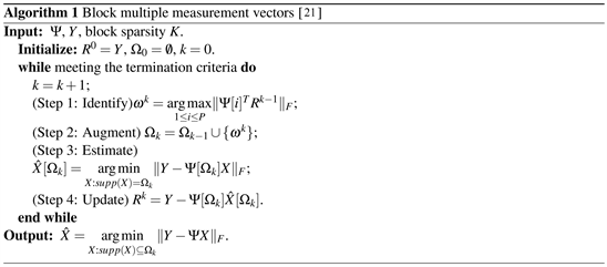
. The BMMV algorithm selects the block index closest to the residual to add to the estimated support at each iteration. The estimated support is used to solve a least square problem to get the estimated original signal. We present the detailed framework of the BMMV algorithm which is described in Algorithm 1.

Like other signal reconstruction algorithms, many results about performance of recovering block MMV problem via BMMV are studied. It is represented in [22] that if Ψ obeys δ K + 1 < 1 K + 1 , then the block K-joint sparse matrices can be accurately reconstructed in K iterations from noiseless model Y = Ψ X by BMMV. In [21] , the condition in [22] was improved to δ K + 1 < 1 K + 1 which also is proved to be sharp. As far as we know, there are no researches on support recovery under noisy model (3) with block structure. We complete this part of content that has not yet been studied. It is necessary to study the recovery performance of the BMMV algorithm in noisy case because it is inevitably contaminated by noise in practical applications. Specifically, we firstly prove that if δ K + 1 < 1 K + 1 and min i Ω X [ i ] F > 2 ε 1 K + 1 δ K + 1 , then the BMMV algorithm can perfectly recover s u p p ( X ) with stopping criteria R k F ε under V F ε . Moreover, our sufficient condition is optimal if noisy model degenerates to noiseless model. Besides, when d = 1 and H = 1 , the BMMV algorithm turns to the OMP algorithm, and the sufficient condition we mentioned above degenerates to ( [17] , Theorem 1).

2. Preliminaries

2.1. Notation

Let 2 and F denote the l 2 and Frobenius norm of a vector and matrix, respectively. The zero and identity matrix are denoted by 0 and I, respectively. The j-th element of vector x is denoted by x j . Let Ω = s u p p ( X ) = { j | X T [ j ] 0 } denotes the support of a matrix X with block structure, then | Ω | K for any matrix X which is block K-joint sparse, where X T [ j ] denote the transpose of X [ j ] . P as the number of blocks of X is assumed for simplity. Let S 1 \ S 2 represents a set which elements are indexed by S 1 and are not contained in set S 2 for any set S 1 , S 2 { 1,2, , P } . Similarly, we use Ω c = { 1,2, , P } \ Ω and Γ c = { 1,2, , P } \ Γ represent the complementary of set Ω and Γ , respectively. Let Ψ [ Γ ] = ( Ψ [ Γ ] T Ψ [ Γ ] ) 1 Ψ [ Γ ] T denotes the pseudoinverse of Ψ [ Γ ] if the rank of the columns of Ψ [ Γ ] is full, where the inverse of a square matrix is represented by ( ) 1 . Therefore, the projector and its orthogonal complement on the columns space of Ψ [ Γ ] can be denoted by P [ Γ ] = Ψ [ Γ ] Ψ [ Γ ] and P [ Γ ] = I P [ Γ ] , respectively.

2.2. Some Useful Lemmas

For proving our subsequent theoretical studies, we first present some useful lemmas for our theoretical analysis.

Lemma 1 ( [26] , Lemma 1) Suppose Ψ obeys both the bRIP of orders K 1 and K 2 , then δ K 1 δ K 2 with K 1 < K 2 .

Lemma 2 ( [11] , Proposition 3.1) Suppose Γ is a set with | Γ | K and Ψ obeys the bRIP of order K. Then

Ψ T [ Γ ] x 2 ( 1 + δ K ) x 2 ,

where x M .

Lemma 3 ( [26] , Lemma 2) Let S 1 and S 2 satisfy | S 1 \ S 2 | 1 . Suppose Ψ obeys | S 1 S 2 | -order bRIP, then

( 1 δ | S 1 S 2 | ) x 2 2 P [ S 1 ] Ψ [ S 2 \ S 1 ] x 2 2 ( 1 + δ | S 1 S 2 | ) x 2 2 ,

where x | S 2 S 1 | .

Lemma 4 ( [27] , Lemma 1) Let B m × n and D n × p . Then

B D F 2 D F B T B D F .

3. Main Results

Lemma 5 is proposed and plays a very important role in the subsequent theoretical proof.

Lemma 5 Let Γ Ω with | Γ | < | Ω | , then

max i Ω \ Γ Ψ T [ i ] P [ Γ ] Ψ [ Ω \ Γ ] X [ Ω \ Γ ] F max j Ω c Ψ T [ j ] P [ Γ ] Ψ [ Ω \ Γ ] X [ Ω \ Γ ] F X [ Ω \ Γ ] F | Ω \ Γ | ( 1 | Ω \ Γ | + 1 δ | Ω | + 1 ) .

Proof 1 The skill of proof is similar to the results in ([21, Lemma 4, Lemma 5). To prove Lemma 5, we first show that

max i Ω \ Γ Ψ T [ i ] P [ Γ ] Ψ [ Ω \ Γ ] X [ Ω \ Γ ] F P [ Γ ] Ψ [ Ω \ Γ ] X [ Ω \ Γ ] F 2 | Ω \ Γ | X [ Ω \ Γ ] F . (6)

By assumption, it is easy to get Γ Ω , | Γ | < | Ω | , and X [ Ω \ Γ ] F 0 , then

max i Ω \ Γ Ψ T [ i ] P [ Γ ] Ψ [ Ω \ Γ ] X [ Ω \ Γ ] F Ψ T [ Ω \ Γ ] P [ Γ ] Ψ [ Ω \ Γ ] X [ Ω \ Γ ] F | Ω \ Γ | = (i) ( P [ Γ ] Ψ T [ Ω \ Γ ] ) P [ Γ ] Ψ [ Ω \ Γ ] X [ Ω \ Γ ] F | Ω \ Γ | (ii) P [ Γ ] Ψ [ Ω \ Γ ] X [ Ω \ Γ ] F 2 | Ω \ Γ | X [ Ω \ Γ ] F ,

(i) is because

( P [ Γ ] ) T P [ Γ ] = P [ Γ ] P [ Γ ] = P [ Γ ] , (7)

and (ii) is from Lemma 4 with B = P [ Γ ] Ψ [ Ω \ Γ ] , and D = X [ Ω \ Γ ] . Thus, (6) holds. So, by (6), we can easily get that

P [ Γ ] Ψ [ Ω \ Γ ] X [ Ω \ Γ ] F 2 | Ω \ Γ | X [ Ω \ Γ ] F max i Ω \ Γ Ψ T [ i ] P [ Γ ] Ψ [ Ω \ Γ ] X [ Ω \ Γ ] F . (8)

Let

α = | Ω \ Γ | + 1 1 | Ω \ Γ | ,

then, by some sample calculations, we obtain

2 α 1 α 2 = | Ω \ Γ | , (9)

1 + α 2 1 α 2 = | Ω \ Γ | + 1 . (10)

To simplify the notation, for given j Ω c , it is necessary to introduce a new matrix Z d × P , and the p-th column of Z is defined as

Z p = Ψ T [ j ] P [ Γ ] Ψ [ Ω \ Γ ] X p [ Ω \ Γ ] Ψ T [ j ] P [ Γ ] Ψ [ Ω \ Γ ] X p [ Ω \ Γ ] F , 1 p P , (11)

where X p [ Ω \ Γ ] is the p-th column of X [ Ω \ Γ ] | Ω \ Γ | × P . Furthermore, we define

Q = P [ Γ ] [ Ψ [ Ω \ Γ ] Ψ [ j ] ] M × ( | Ω \ Γ | + 1 ) , (12)

U = [ X [ Ω \ Γ ] 0 ] ( | Ω \ Γ | + 1 ) × P , (13)

W = [ 0 α X [ Ω \ Γ ] F Z ] ( | Ω \ Γ | + 1 ) × P . (14)

Then

Q U = P [ Γ ] Ψ [ Ω \ Γ ] X [ Ω \ Γ ] (15)

and

U + W F 2 = ( 1 + α 2 ) X [ Ω \ Γ ] F 2 , (16)

α 2 U W F 2 = α 2 ( 1 + α 2 ) X [ Ω \ Γ ] F 2 . (17)

Moreover,

p = 1 P W i T Q T Q U i = (iii) α X [ Ω \ Γ ] F p = 1 P Z p T Ψ T [ j ] P [ Γ ] P [ Γ ] Ψ [ Ω \ Γ ] X p [ Ω \ Γ ] = (iv) α X [ Ω \ Γ ] F p = 1 P Z p T Ψ T [ j ] P [ Γ ] Ψ [ Ω \ Γ ] X p [ Ω \ Γ ] = (v) α X [ Ω \ Γ ] F Ψ T [ j ] P [ Γ ] Ψ [ Ω \ Γ ] X p [ Ω \ Γ ] F , (18)

where (iii) is because (12)-(15), (iv) follows from (7), and (v) is from (11). Therefore, for any j Ω c , by applying (18), we can get

Q ( U + W ) F 2 = p = 1 P Q ( U p + W p ) 2 2 = p = 1 P ( Q U p 2 2 + Q W p 2 2 ) + 2 p = 1 P W p T Q T Q U p = Q U F 2 + Q W F 2 + 2 α X [ Ω \ Γ ] F Ψ T [ j ] P [ Γ ] Ψ [ Ω \ Γ ] X [ Ω \ Γ ] F (19)

and

Q ( α 2 U W ) F 2 = p = 1 P Q ( α 2 U p W p ) 2 2 = p = 1 P ( α 4 Q U p 2 2 + Q W p 2 2 ) 2 α 2 p = 1 P W p T Q T Q U p = α 4 Q U F 2 + Q W F 2 2 α 3 X [ Ω \ Γ ] F Ψ T [ j ] P [ Γ ] Ψ [ Ω \ Γ ] X [ Ω \ Γ ] F . (20)

By the (19) and (20) are mentioned before, we can have

Q ( U + W ) F 2 Q ( α 2 U W ) F 2 = ( 1 α 4 ) Q U F 2 + 2 α ( 1 + α 2 ) X [ Ω \ Γ ] F Ψ T [ j ] P [ Γ ] Ψ [ Ω \ Γ ] X [ Ω \ Γ ] F = ( 1 α 4 ) ( Q U F + 2 α 1 α 2 × X [ Ω \ Γ ] F Ψ T [ j ] P [ Γ ] Ψ [ Ω \ Γ ] X [ Ω \ Γ ] F ) = ( 1 α 4 ) ( Q U F | Ω \ Γ | × X [ Ω \ Γ ] F Ψ T [ j ] P [ Γ ] Ψ [ Ω \ Γ ] X [ Ω \ Γ ] F ) , (21)

where the last equality because of (9). It is not hard to check that

Q ( U + W ) F 2 Q ( α 2 U W ) F 2 ( vi ) ( 1 δ | Ω | + 1 ) U + W F 2 ( 1 + δ | Ω | + 1 ) α 2 U W F 2 = ( vii ) ( 1 δ | Ω | + 1 ) ( 1 + α 2 ) X [ Ω \ Γ ] F 2 ( 1 + δ | Ω | + 1 ) α 2 ( 1 + α 2 ) X [ Ω \ Γ ] F 2 = ( 1 + α 2 ) X [ Ω \ Γ ] F 2 ( ( 1 δ | Ω | + 1 ) ( 1 + δ | Ω | + 1 ) α 2 )

= ( 1 + α 2 ) X [ Ω \ Γ ] F 2 ( ( 1 α 2 ) δ | Ω | + 1 ( 1 + α 2 ) ) = ( 1 α 4 ) X [ Ω \ Γ ] F 2 ( 1 1 + α 2 1 α 2 δ | Ω | + 1 ) = ( viii ) ( 1 α 4 ) X [ Ω \ Γ ] F 2 ( 1 | Ω \ Γ | + 1 δ | Ω | + 1 ) , (22)

where (vi) follows Lemma 3 and (12), (vii) is due to (16) and (17), and (viii) is from (10). By (15), (21), (22), and the fact that 1 α 4 > 0 , we have

P [ Γ ] Ψ [ Ω \ Γ ] X [ Ω \ Γ ] F 2 | Ω \ Γ | X [ Ω \ Γ ] F Ψ T [ j ] P [ Γ ] Ψ [ Ω \ Γ ] X [ Ω \ Γ ] F = Q U F 2 | Ω \ Γ | X [ Ω \ Γ ] F Ψ T [ j ] P [ Γ ] Ψ [ Ω \ Γ ] X [ Ω \ Γ ] F X [ Ω \ Γ ] F 2 ( 1 | Ω \ Γ | + 1 δ | Ω | + 1 ) .

Combining the aforementioned Equation with (8), we obtain

| Ω \ Γ | X [ Ω \ Γ ] F × ( max i Ω \ Γ Ψ T [ i ] P [ Γ ] Ψ [ Ω \ Γ ] X [ Ω \ Γ ] F Ψ T [ j ] P [ Γ ] Ψ [ Ω \ Γ ] X [ Ω \ Γ ] F ) | Ω \ Γ | X [ Ω \ Γ ] F × ( max i Ω \ Γ Ψ T [ i ] P [ Γ ] Ψ [ Ω \ Γ ] X [ Ω \ Γ ] F

max j Ω c Ψ T [ j ] P [ Γ ] Ψ [ Ω \ Γ ] X [ Ω \ Γ ] F ) X [ Ω \ Γ ] F 2 ( 1 | Ω \ Γ | + 1 δ | Ω | + 1 ) ,

which implies that

max i Ω \ Γ Ψ T [ i ] P [ Γ ] Ψ [ Ω \ Γ ] X [ Ω \ Γ ] F max j Ω c Ψ T [ j ] P [ Γ ] Ψ [ Ω \ Γ ] X [ Ω \ Γ ] F ( 1 | Ω \ Γ | + 1 δ | Ω | + 1 ) X [ Ω \ Γ ] F | Ω \ Γ | .

Thus, we complete the proof.

Remark 6 Specially, Lemma 5 is a general block version of ( [28] , Theorem 3.2). The main difference between our Lemma 5 and ( [28] , Theorem 3.2) exist in two aspects. First, our model is block version of multiple measurement vectors. Second, the ways of calculating s u p p ( X ) are different.

Based on the Algorithm 1 and lemmas we presented above, we show our main results in this section. We provide a sufficient guarantee for the exact support recovery of block joint sparse matrices with the BMMV algorithm under the V F ε bounded noise from noisy model (3).

Theorem 7 Consider (3). Assume that V F ε and matrix X is block K-joint sparse. Provided that measurement matrix Ψ obeys the bRIP of order K + 1 with

δ K + 1 < 1 K + 1 , (23)

and X satisfies

min i Ω X [ i ] F > 2 ε 1 K + 1 δ K + 1 . (24)

Then based on the stopping criteria R k F ε , the BMMV algorithm can accurately recover the s u p p ( X ) in K iterations.

Proof 2 For proving Theorem 7, there are two points that need to be shown, namely, one is to prove that the BMMV algorithm selects a correct block index from Ω = s u p p ( X ) in each iteration, and the second is that the BMMV algorithm will select all the indices in Ω in all K iterations. The proof consists of two parts. First, we illustrate that all correct indices are identified in all iteration via BMMV. Second, we show that the process of identifying terminates after it is executed just K = | Ω | iterations. In the first step the mathematical induction method is used. Suppose that in the first k 1 iterations, the BMMV algorithm has selected the correct indices, which means that Ω k 1 = { ω 1 , ω 2 , , ω k 1 } Ω and 1 k | Ω | = K . Since Ω 0 = , it obviously holds when k = 1 . Therefore, we only have to prove that a correct index is selected by the BMMV algorithm at the k-th iteration, i.e., ω k Ω \ Ω k 1 .

By the Step 3 and 4 in Algorithm 1, we can obtain that the orthogonal relationship between R k 1 and the columns space of Ψ [ i ] , then we have

Ψ T [ i ] R k 1 F = 0,

for any i Ω k 1 , so we get that ω k Ω k 1 . For proving ω k Ω \ Ω k 1 , by the Step 1 of BMMV, we turn to proof

max i Ω \ Ω k 1 Ψ T [ i ] R k 1 F > max j Ω c Ψ T [ j ] R k 1 F . (25)

By the estimating step of the BMMV algorithm, we obtain

X ^ [ Ω k 1 ] = ( Ψ T [ Ω k 1 ] Ψ [ Ω k 1 ] ) 1 Ψ T [ Ω k 1 ] Y . (26)

Then, from Step 4 of the BMMV algorithm and (26),

R k 1 = Y Ψ [ Ω k 1 ] X ^ [ Ω k 1 ] = ( τ 1) P [ Ω k 1 ] ( Ψ X + V ) = ( τ 2) P [ Ω k 1 ] ( Ψ [ Ω k 1 ] X [ Ω k 1 ] + Ψ [ Ω \ Ω k 1 ] X [ Ω \ Ω k 1 ] + V ) = ( τ 3) P [ Ω k 1 ] Ψ [ Ω \ Ω k 1 ] X [ Ω \ Ω k 1 ] + P [ Ω k 1 ] V , (27)

where (τ1) is because the definition of P [ Ω k 1 ] is used, (τ2) is based on Ω = s u p p ( X ) and Ω k 1 Ω , and (τ3) is due to P [ Ω k 1 ] Ψ [ Ω k 1 ] = 0 . Consequently, to show (25), we try to use (27) to obtain the lower and upper bound on the left and right side of (25), separately. For any i Ω \ Ω k 1 and j Ω c , by the triangle inequality, it is obtained that

max i Ω \ Ω k 1 Ψ T [ i ] R k 1 F = max i Ω \ Ω k 1 Ψ T [ i ] P [ Ω k 1 ] Ψ [ Ω \ Ω k 1 ] X [ Ω \ Ω k 1 ] + Ψ T [ i ] P [ Ω k 1 ] V F max i Ω \ Ω k 1 Ψ T [ i ] P [ Ω k 1 ] Ψ [ Ω \ Ω k 1 ] X [ Ω \ Ω k 1 ] F max i Ω \ Ω k 1 Ψ T [ i ] P [ Ω k 1 ] V F (28)

and

max j Ω c Ψ T [ j ] R k 1 F = max j Ω c Ψ T [ j ] P [ Ω k 1 ] Ψ [ Ω \ Ω k 1 ] X [ Ω \ Ω k 1 ] + Ψ T [ j ] P [ Ω k 1 ] V F max j Ω c Ψ T [ j ] P [ Ω k 1 ] Ψ [ Ω \ Ω k 1 ] X [ Ω \ Ω k 1 ] F max j Ω c Ψ T [ j ] P [ Ω k 1 ] V F . (29)

Therefore, by (28) and (29), to show (25), we only need to prove

max i Ω \ Ω k 1 Ψ T [ i ] P [ Ω k 1 ] Ψ [ Ω \ Ω k 1 ] X [ Ω \ Ω k 1 ] F max j Ω c Ψ T [ j ] P [ Ω k 1 ] Ψ [ Ω \ Ω k 1 ] X [ Ω \ Ω k 1 ] F > max i Ω \ Ω k 1 Ψ T [ i ] P [ Ω k 1 ] V F + max j Ω c Ψ T [ j ] P [ Ω k 1 ] V F . (30)

Next, we try to find a lower bound on the left side of (30). Using the inductive assumption Ω k 1 Ω and | s u p p ( X [ Ω \ Ω k 1 ] ) | = | Ω | + 1 k . Hence, we obtain

X [ Ω \ Ω k 1 ] F | Ω | + 1 k min i Ω X [ i ] F . (31)

Since | Ω k 1 | = k 1 and Ω k 1 Ω , according to Lemma 5, we obtain

max i Ω \ Ω k 1 Ψ T [ i ] P [ Ω k 1 ] Ψ [ Ω \ Ω k 1 ] X [ Ω \ Ω k 1 ] F max j Ω c Ψ T [ j ] P [ Ω k 1 ] Ψ [ Ω \ Ω k 1 ] X [ Ω \ Ω k 1 ] F X [ Ω \ Ω k 1 ] F | Ω | + 1 k ( 1 | Ω | + 2 k δ | Ω | + 1 ) ( τ 4) X [ Ω \ Ω k 1 ] F | Ω | + 1 k ( 1 K + 1 δ | Ω | + 1 ) ( τ 5) min i Ω X [ i ] F ( 1 K + 1 δ K + 1 ) , (32)

where (τ4) is due to the assumption of X in this paper and the fact that k > 1 and (τ5) is from Lemma 1, (23) and (31). Then, we deduce a upper bound on the right side of (30). There are α Ω \ Ω k 1 and β Ω c that make

max i Ω \ Ω k 1 Ψ T [ i ] P [ Ω k 1 ] V F = Ψ T [ α ] P [ Ω k 1 ] V F ,

max j Ω c Ψ T [ j ] P [ Ω k 1 ] V F = Ψ T [ β ] P [ Ω k 1 ] V F .

Hence, we obtain

max i Ω \ Ω k 1 Ψ T [ i ] P [ Ω k 1 ] V F F + max j Ω c Ψ T [ j ] P [ Ω k 1 ] V F = Ψ T [ α ] P [ Ω k 1 ] V F + Ψ T [ β ] P [ Ω k 1 ] V F ( τ 6) 2 [ Ψ [ α ] , Ψ [ β ] ] T P [ Ω k 1 ] V F ( τ 7) 2 ( 1 + δ K + 1 ) ε , (33)

where (τ6) is because [ Ψ [ α ] , Ψ [ β ] ] T P [ Ω k 1 ] V is a matrix with two d × H subvectors and (τ7) are due to Lemma 2 and

P [ Ω k 1 ] V F V F ε , (34)

respectively. Based on (32) and (33), (30) holds when

2 ( 1 + δ K + 1 ) ε < ( 1 K + 1 δ K + 1 ) min i Ω X [ i ] F ,

that is,

min i Ω X [ i ] F > 2 ( 1 + δ K + 1 ) ε 1 K + 1 δ K + 1 .

In addition, by (23), we obtain δ K + 1 < 1 . Hence, once (24) is satisfied, a correct index is identified by the BMMV algorithm in each iteration.

Next, the BMMV algorithm needs to be specified to be performed exact | Ω | = K iterations, that equals to prove that we always have R k F > ε for all k [ 1, K ) and R K F ε . Since only one correct index is selected by the BMMV algorithm at a iteration under (24), by (27) and triangle inequality, for all k [ 1, K ) , we obtain

R k F = P [ Ω k ] Ψ [ Ω \ Ω k ] X [ Ω \ Ω k ] + P [ Ω k ] V F P [ Ω k ] Ψ [ Ω \ Ω k ] X [ Ω \ Ω k ] F P [ Ω k ] V F ( τ 8) 1 δ K X [ Ω \ Ω k ] F ε ( τ 9) ( 1 δ K + 1 ) ( K k ) min i Ω X [ i ] F ε 1 δ K + 1 ε ,

where (τ8) is from (34) and Lemma 3, and (τ9) is because of Lemma 1 and (31). Hence, if

min i Ω X [ i ] F > 2 ε 1 δ K + 1 , (35)

then R k F > ε for each k [ 1, K ) . After some transformations, it is easily get

2 ε 1 K + 1 δ K + 1 2 ε 1 δ K + 1 , (36)

which is from 1 δ K + 1 ( 0,1 ) and 1 K + 1 δ K + 1 1 δ K + 1 . Therefore, from (35) and (36), if (24) holds, R k F > ε for each 1 k < K , i.e., it does not terminate until the K-th iteration is completed. Likewise, from (27), we have

R K F = P [ Ω K ] Ψ [ Ω \ Ω K ] X [ Ω \ Ω K ] + P [ Ω K ] V F = ( τ 10) P [ Ω K ] V F ε ,

where (τ10) is due to | Ω K | = | Ω | = K . Due to the termination criteria, the BMMV algorithm stops after the K-th iteration. Hence, the BMMV algorithm just executes K iterations. Our proof is complete.

When H = 1 , the X turns to a block K-sparse vector x and V turns to a vector v . For block K-sparse vector, there are already many researches on recovery performance of block reconstruction algorithms, for example, block OMP (BOMP) ( [26] [29] ) and block gOMP (BgOMP) ( [30] [31] ).

Corollary 8 Taking H = 1 in (3) and Theorem 7. Assume that v 2 ε and vector x is block K sparse. Provided that measurement matrix Ψ obeys the bRIP of order K + 1 with δ K + 1 < 1 K + 1 , and x satisfies

min i Ω x [ i ] 2 > 2 ε 1 K + 1 δ K + 1 .

Then based on the stopping criteria r k 2 ε ( r is a residual vector), the BMMV algorithm can accurately recover s u p p ( x ) in K iterations.

Remark 9 The results in the Corollary 8 are consistent with the results of [26] , which is a sharp sufficient condition. However, [29] gives a new analysis for support recovery that is less restrictive for min i Ω x [ i ] 2 . For more details, please refer to [29] .

If the length of blocks d = 1 , the block K-joint sparse is equivalent to K-row sparse. In [32] gives two theorems to show the bound δ K + 1 < 1 K + 1 is optimal in noiseless case. More details are in [32] , which means the bound based on bRIP we proposed is optimal in the noiseless case.

Corollary 10 Taking H = 1 and d = 1 in (3) and Theorem 7, X reduces to x , V reduces to v . Assume that v 2 ε and vector x is K sparse. Provided that measurement matrix Ψ obeys the bRIP of order K + 1 with δ K + 1 < 1 K + 1 , and x satisfies

min i Ω | x i | > 2 ε 1 K + 1 δ K + 1 .

Then based on the stopping criteria r k 2 ε , the BMMV algorithm can accurately recover s u p p ( x ) in K iterations.

Remark 11 The Corollary 10 is same as ( [17] , Theorem 1), which is a sharp condition. [33] gives a less restrictive bound on min i Ω | x i | . This means that our result have room for improvement.

4. Conclusions and Future Works

In this paper, studies on the performance of support recovery of block K-joint sparse matrix via the BMMV algorithm from Y = Ψ X + V are analyzed. We obtained that if Ψ satisfies bRIP with δ K + 1 < 1 K + 1 and min i Ω X [ i ] F 2 ε 1 K + 1 δ K + 1 , then BMMV can accurately reconstruct the s u p p ( X ) in K iterations. With the help of ( [32] , Theorem 2), we also show the RIP-based condition is optimal when the problem reduces to SMV problem under the noiseless case.

Because our result about min i Ω X [ i ] F is not yet optimal. Thus, one of future directions is to continue to refine this result and continue to study theoretical improvement of the related algorithms. Because the block length considered in this paper is a fixed value for simplicity, it is also worth considering that the block length is a variable. Then, the support recovery conditions are theoretical, and how it applies to practical applications is also a question. The BMMV algorithm selects only one index for each iteration, which means that the recovery program will directly fail once a wrong index is added to the estimation support. It is interesting to propose an improved algorithm to solve the problem.

Conflicts of Interest

The authors declare no conflicts of interest regarding the publication of this paper.

References

[1] Candes, E.J., Romberg, J. and Tao, T. (2006) Robust Uncertainty Principles: Exact Signal Reconstruction from Highly Incomplete Frequency Information. IEEE Transactions on Information Theory, 5, 489-509.
https://doi.org/10.1109/TIT.2005.862083
[2] Donoho, D.L. (2006) Compressed Sensing. IEEE Transactions on Information Theory, 52, 1289-1306.
https://doi.org/10.1109/TIT.2006.871582
[3] Duarte, M.F. and Eldar, Y.C. (2011) Structured Compressed Sensing: From Theory to Applications. IEEE Transactions on Information Theory, 59, 4053-4085.
https://doi.org/10.1109/TSP.2011.2161982
[4] Donoho, D.L., Elad, M. and Temlyakov V. (2006) Stable Recovery of Sparse Overcomplete Repesentations in the Presence of Noise. IEEE Transactions on Information Theory, 52, 6-18.
https://doi.org/10.1109/TIT.2005.860430
[5] Herman, M. and Strohmer, T. (2009) High-Resolution Radar via Compressed Sensing. IEEE Transactions Signal Processing, 57, 2275-2284.
https://doi.org/10.1109/TSP.2009.2014277
[6] Lustig, M., Donoho, D.L. and Pauly, J.M. (2008) Compressed Sensing MRI. IEEE Signal Processing Magazine, 25, 72-82.
https://doi.org/10.1109/MSP.2007.914728
[7] Wakin, M., Laska, J., Duarte, M., et al. (2006) An Architecture for Compressive Imaging. 2006 International Conference on Image Processing, Atlanta, 8-11 October 2006, 1273-1276.
https://doi.org/10.1109/ICIP.2006.312577
[8] Tropp, J.A. and Gilbert, A.C. (2007) Signal Recovery from Random Measurements via Orthogonal Matching Pursuit. IEEE Transactions on Information Theory, 53, 4655-4666.
https://doi.org/10.1109/TIT.2007.909108
[9] Donoho, D.L., Tsaig, Y., Drori, I. and Starck, J.L. (2012) Sparse Solution of Underdetermined Systems of Linear Equations by Stagewise Orthogonal Matching Pursuit. IEEE Transactions on Information Theory, 58, 1094-1121.
https://doi.org/10.1109/TIT.2011.2173241
[10] Needell, D. and Vershynin, R. (2009) Uniform Uncertainty Principle and Signal Recovery via Regularized Orthogonal Matching Pursuit. Foundations of Computational Mathematics, 9, 317-334.
https://doi.org/10.1007/s10208-008-9031-3
[11] Needell, D. and Tropp, J.A. (2009) CoSaMP: Iterative Signal Recovery from Incomplete and Inaccurate Samples. Applied and Computational Harmonic Analysis, 26, 301-321.
https://doi.org/10.1016/j.acha.2008.07.002
[12] Dai, W. and Milenkovic, O. (2009) Subspace Pursuit for Compressive Sensing Signal Reconstruction. IEEE Transactions on Information Theory, 55, 2230-2249.
https://doi.org/10.1109/TIT.2009.2016006
[13] Wang, J., Kwon, S. and Shim, B. (2012) Generalized Orthogonal Matching Pursuit. IEEE Transactions Signal Processing, 60, 6202-6216.
https://doi.org/10.1109/TSP.2012.2218810
[14] Rebollo-Neira, L. and Lowe, D. (2002) Optimized Orthogonal Matching Pursuit Approach. IEEE Signal Processing Letters, 9, 137-140.
https://doi.org/10.1109/LSP.2002.1001652
[15] Huang, H. and Makur, A. (2011) Backtracking-Based Matching Pursuit Method for Sparse Signal Reconstruction. IEEE Signal Processing Letters, 18, 391-394.
https://doi.org/10.1109/LSP.2011.2147313
[16] Mo, Q. and Shen, Y. (2012) A Remark on the Restricted Isometry Property in Orthogonal Matching Pursuit. IEEE Transactions on Information Theory, 58, 3654-3656.
https://doi.org/10.1109/TIT.2012.2185923
[17] Wen, J.M., Zhou, Z.C., Wang, J., Tang, X.H. and Mo, Q. (2017) A Sharp Condition for Exact Support Recovery with Orthogonal Matching Pursuit. IEEE Transactions Signal Processing, 65, 1370-1382.
https://doi.org/10.1109/TSP.2016.2634550
[18] Wang, J., Zhou, Z., Li, D. and Tang, X. (2016) A Novel Sufficient Condition for Generalized Orthogonal Matching Pursuit. IEEE Communications Letters, 21, 805-808.
https://doi.org/10.1109/LCOMM.2016.2642922
[19] Mishali, M. and Eldar, Y.C. (2009) Blind Multiband Signal Reconstruction: Compressed Sensing for Analog Signals. IEEE Transactions Signal Processing, 57, 993-1009.
https://doi.org/10.1109/TSP.2009.2012791
[20] Wright, J., Yang, A.Y., Granesh, A., Sastry, S.S. and Ma, Y. (2009) Robust Face Recognition via Sparse Representation. IEEE Transactions on Pattern Analysis and Machine Intelligence, 31, 210-227.
https://doi.org/10.1109/TPAMI.2008.79
[21] Shi, Y.L., Wang, L.B. and Luo, R. (2019) Sparse Recovery with Block Multiple Measurement Vectors Algorithm. IEEE Access, 7, 9470-9475.
https://doi.org/10.1109/ACCESS.2019.2891568
[22] Fu, Y., Li, H., Zhang, Q. and Zhou, J. (2014) Block-Sparse Recovery via Redundant Block OMP. Signal Precessing, 97, 162-171.
https://doi.org/10.1016/j.sigpro.2013.10.030
[23] Candes, E.J. and Tao, T. (2005) Denoding by Linear Programming. IEEE Transactions on Information Theory, 51, 4203-4215.
https://doi.org/10.1109/TIT.2005.858979
[24] Robust, Y.C. and Mishali, M. (2009) Robust Recovery of Signals from a Structured Union of Subspaces. IEEE Transactions on Information Theory, 55, 5302-5316.
https://doi.org/10.1109/TIT.2009.2030471
[25] Majumdar, A. and Ward, R.K. (2012) Face Recognition from Video: An MMV Recovery Approach. 2012 IEEE International Conference on Acoustics, Speech and Signal Processing (ICASSP), Kyoto, 25-30 March 2012, 2221-2224.
https://doi.org/10.1109/ICASSP.2012.6288355
[26] Wen, J.M., Zhou, Z.C., Liu, Z.L., Lai, M.J. and Tang, X.H. (2019) Sharp Sufficient Conditions for Stable Recovery of Block Sparse Signals by Block Orthogonal Matching Pursuit. Applied and Computational Harmonic Analysis, 47, 948-974.
https://doi.org/10.1016/j.acha.2018.02.002
[27] Wen, J.M., Tang, J. and Zhou, F.M. (2017) Greedy Block Coordinate Descent under Restricted Isometry Property. Mobile Networks and Applications, 22, 371-376.
https://doi.org/10.1007/s11036-016-0774-9
[28] Zhang, X.W., Xie, L.J. and Wang, J.P. (2022) Some Results on OMP Algorithm for MMV Problem. Mathematical Methods in the Applied Sciences, 45, 5402-5411.
https://doi.org/10.1002/mma.8114
[29] Li, H.F. and Wen, J.M. (2018) A New Analysis for Support Recovery with Block Orthogonal Matching Pursuit. IEEE Signal Processing, 26, 247-251.
https://doi.org/10.1109/LSP.2018.2885919
[30] Qi, R., Yang, D.W., Zhang, Y.J. and Li, H.W. (2018) On Recovery of Block Sparse Signals via Block Generalized Orthogonal Matching Pursuit. Signal Progressing, 153, 34-46.
https://doi.org/10.1016/j.sigpro.2018.06.023
[31] Xia, C.Y., Zhou, Z.L., Guo, C.B., Hao, Y.S. and Hou, C.B. (2021) A New Analysis for Support Performance with Block Generalized Orthogonal Matching Pursuit. Mathematical Problems in Engineering, 2021, Article ID: 9438793.
https://doi.org/10.1155/2021/9438793
[32] Li, H.F., Wang, L.B., Zhan, X.Q. and Jain, D.K. (2019) On the Fundamental Limit of Orthogonal Matching Pursuit for Multiple Measurement Vector. IEEE Access, 7, 48860-48866.
https://doi.org/10.1109/ACCESS.2019.2907684
[33] Liu, C., Fang, Y. and Liu, J.Z. (2017) Some New Results about Sufficient Conditions for Exact Support Recovery of Sparse Signals via Orthogonal Matching Pursuit. IEEE Transactions Signal Processing, 65, 4511-4524.
https://doi.org/10.1109/TSP.2017.2711543

Copyright © 2024 by authors and Scientific Research Publishing Inc.

Creative Commons License

This work and the related PDF file are licensed under a Creative Commons Attribution 4.0 International License.