Regional Boundary Observability with Constraints of the Gradient ()
1. Introduction
For a distributed parameter system evolving on a special domain Ω, the observability concept has been widely developed and survey of these developments can be found [1-3]. Later, the regional observability notion was introduced, and interesting results have been obtained [4,5], in particular, the possibility to observe a state only on a subregion  interior to Ω. These results have been extended to the case where
  is a part of the boundary
  of Ω [6]. Then the concepts of regional gradient observability and regional observability with constraints were introduced and developed by [7-11] in the case where the subregion is interior to Ω and the case where the subregion is a part of
 . Here we are interested to approach the initial state gradient and the reconstructed state between two prescribed functions given only on a boundary subregion
  of system evolution domain. There are many reasons motivating this problem: first the mathematical model of system is obtained from measurements or from approximation techniques and is very often affected by perturbations. Consequently, the solution of such a system is approximately known, and second, in various real problems the target required to be between two bounds. This is the case, for example of a biological reactor “Figure 1” in which the concentration regulation of a substrate at the bottom of the reactor is observed between two levels.
The paper is organized as follows: first we provide results on regional observability for distributed parameter system of parabolic type and we give definitions related to regional boundary observability with constraints of the gradient of parabolic systems. The next section is focused on the reconstruction of the initial state gradient by using an approach based on sub-differential tools. The same objective is achieved in Section 4 by applying the multiplier Lagrangian approach which gives a practice algorithm. The last section is devoted to compute the obtained algorithm with numerical example and simulations.

Figure 1. Regulation of the concentration flux of the substratum at a bottom of the reactor.
2. Problem Statement
Let Ω be an open bounded subset of IRn (n = 2, 3) with regular boundary  and a boundary subregion
  of
of . For a given time
 , let
, let  and
and .
.
Consider a parabolic system defined by
 (1)
(1)
with the measurements given by the output function
 (2)
(2)
where  is linear and depends on the considered sensors structure.
The observation space is .
.
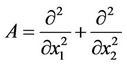
A is a second order differential linear and elliptic operator which generates a strongly continuous semigroup

in the Hilbert space .
.
A denotes the adjoint operators of A.
The initial state  and its gradient
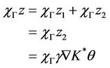
  are assumeed to be unknown. The system (1) is autonomous and (2) allows writing
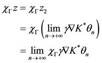
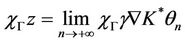
We define the operator

which is linear bounded with the adjoint K* given by

Consider the operator

While  denotes its adjoint given by
where v is a solution of the Dirichlet’s problem

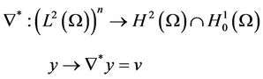
Let

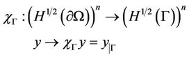
With  is the extension of the trace operator of order zero which is linear and surjective.
 ,
,  denotes the adjoint operators of
  and
and .
.
For , we consider
while  denotes its adjoint.
We recall the following definitions
Definition 2.1
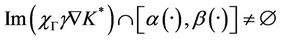
1. The system (1) together with the output (2) is said to be exactly (respectively weakly) gradient observable on Γ if

(respectively  ).
).
2. The sensor (D, f) (or a sequence of sensors) is said to be gradient strategic on Γ if the observed system is weakly gradient observable on Γ.
For more details, we refer the reader to [11].
Let  and
and  be two functions defined in
  such that
  a.e. on Γ for all
 . In the sequel we set

Definition 2.2
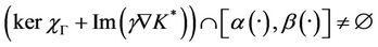
1). The system (1) together with the output (2) is said to be exactly  -gradient observable on Γ if
 .
.
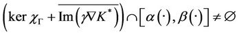
2). The system (1) together with the output (2) is said to be weakly  -gradient observable on Γ if
 .
.
3). A sensor (D, f) is said to be  -gradient strategic on Γ if the observed system is weakly
  -gradient observable on Γ.
Remark 2.3
1). If the system (1) together with the output (2) is exactly  -gradient observable on Γ then it is weakly
  -gradient observable on Γ.
2). If the system (1) together with the output (2) is exactly gradient observable on Γ then it is exactly  -gradient observable on Γ.
3). If the system (1) together with the output (2) is exactly (resp. weakly)  -gradient observable on Γ1 then it is exactly (resp. weakly)
  -gradient observable on any
 .
.
There exist systems which are not weakly gradient observable on a subregion Γ but which are weakly  -gradient observable on Γ.
Example 2.4
Consider the two-dimensional system described by the diffusion equation
 (3)
(3)
where , the time interval is ]0, T[ and let Γ be the boundary subregion given by
 . We consider the sensor (D, f) defined by
 and
and
 .
.
Thus, the output function is given by
 (4)
(4)
The operator
generates a semigroup  in
in  given by
 (5)
(5)
where 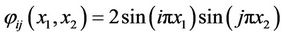
and  .
.
Then we have the result:
Proposition 2.5
The system (3) together with the output (4) is not weakly gradient observable on Γ but it is weakly  -gradient observable on Γ.
Proof
Let g1 be the function defined in Ω by

be the gradient to be observed on Γ and show that g1 is not weakly gradient observable on Γ.
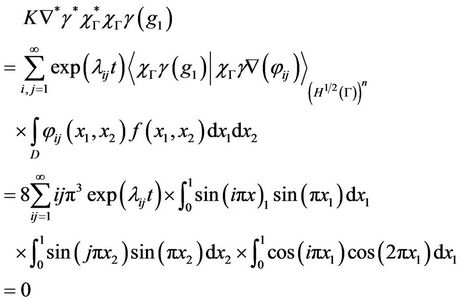
we have . Consequently, the gradient g1 is not weakly gradient observable on Γ. Then the system (3) together with the output (4) is not weakly gradient observable on Γ. but we can show that it is weakly
  -gradient observable on Γ, indeed, for

we have
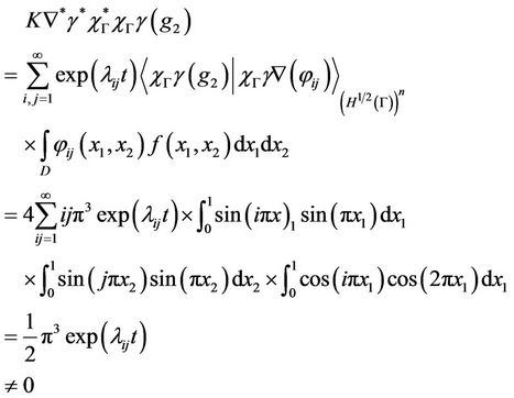
which show that the gradient g2 is weakly gradient observable on Γ.
For  and
and , we have that
 , then the system (3) together with the output (4) is weakly
  -gradient observable on Γ.
Proposition 2.6
The system (1) together with the output (2) is exactly  -gradient observable on Γ if and only if

Proof
- If 
then, we can find  such that
 then
then  where
where  and
and  with
with , then
and  thus
thus
which shows that the system (1) together with the output (2) is exactly  -gradient observable on Γ.
- Assume that the system (1) together with the output (2) is exactly  -gradient observable on Γ, which is equivalent to

then there exists  and
and  such that
  which gives
 .
.
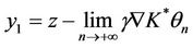
Let  and
and , then z = y1 + y2 with
  and
and  which shows that

and therefore
Proposition 2.7
The system (1) together with the output (2) is weakly  -gradient observable on Γ if and only if

Proof
- Suppose that
then, there exists  such that

so , where
  and
and
with ,
,  , then
and

therefore
which implies that the system (1) together with the output (2) is weakly  -gradient observable on Γ.
- Suppose that the system (1) together with the output (2) is weakly  -gradient observable on Γ, which is equivalent to

then there exists  and
and  a sequence of elements of
  .such that
which gives
 .
.
Let
and
 then
then  with
with  and
and

which shows that
and therefore

3. Subdifferential Approach
This section is focused on the characterization of the initial state of the system (1) together with the output (2) in the nonempty subregion Γ with constraints on the gradient by using an approach based on subdifferential tools [12]. So we consider the optimization problem
 (6)
(6)
where

Let us denote by
-  the set of functions

proper, lower semi-continuous (l.s.c.) and convex.
- For  the polar function f* of f be given by

where
 .
.
- For  the set
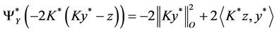
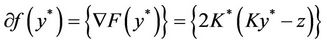

denotes the subdifferential of f at y0, then we have  if and only if
 .
.
- For D a nonempty subset of 
denotes the indicator functional of D.
With these notations the problem (6) is equivalent to the problem:
 (7)
(7)
The solution of this problem may be characterized by the following result.
Proposition 3.1
If the system (1) together with the output (2) is exactly  -gradient observable on Γ, then y* is a solution of (7) if and only if
  and
and
Proof
We have that y* is a solution of (7) if and only if
 with
with
 since
since
 Y is closed, convex and nonempty, then

Also, according to the hypothesis of the  - gradient observability on Γ, we have
 .
.
Now F is continuous, then

it follows that y* is a solution of (7) if and only if
 .
.
On the other hand F is Frechet-differentiable, then
and y* is a solution of (7) if and only if
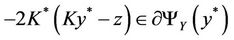
which is equivalent to  and
and

and consequently  and
and

4. Lagrangian Multiplier Approach
In this section we propose to solve the problem (6) using the Lagrangian multiplier method [13]. Also we describe a numerical algorithm which allows the computation of the initial state gradient on the boundary subregion Γ and finally we illustrate the obtained results by numerical simulation which tests the efficiency of the numerical scheme.
From the definition of the exact  -gradient observability on Γ all state we will consider are of the form
  such that
 . So the last minimization problem is equivalent to
 (8)
(8)
with
 .
.
Then we have the following result:
Proposition 4.1
If the system (1) together with the output (2) is exactly observable in Ω, exactly  -boundary gradient observable on Γ with
 ,
,  ,
,  then the solution of (8) is given by
 (9)
(9)
and the gradient in Γ of the solution of the problem (6) is given by
 (10)
(10)
where  is the solution of
 (11)
(11)
while
 denotes the projection operator,
  and
and
 .
.
Proof
The system (1) together with the output (2) is  -gradient observable on Γ then
  and the problem (8) has a solution. The problem (8) is equivalent to the saddle point problem
 (12)
(12)
where

We associate with problem (12) the Lagrangian functional L defined by the formula

for all
 .
.
Let us recall that  is a saddle point of L if
- 
- The system (1) together with the output (2) is  -gradient observable on Γ and, therefore, there exist
  and
and  such that
 which implies
 as
as

moreover, there exists  such that

then L admits a saddle point.
- Let  be a saddle point of L and prove that
  is the restriction gradient on Γ of the solution of (6).
We have
for all
 .
.
The first inequality above gives

 .
.
which implies that  and hence
 .
.
The second inequality means that
we have
 .
.
Since  we have
for all
 .
.
Taking
 we obtain

which implies that  minimize
 , and so
  whose the restriction of the gradient on Γ is
  minimize the function
  for all the states which are of the form
  with
with .
.
- Now if  is a saddle point of L, then the following assumptions hold
 (13)
(13)
 (14)
(14)
 (15)
(15)
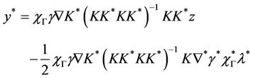
From (13) we have

Then

we assume that the system is observable in Ω, then  is invertible, and

so y* is given by

Then
with
 .
.
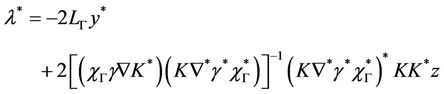
By (14) we have

Then

Corollary 4.2
If the system (1) together with the output (2) is observable in Ω, exactly gradient observable on Γ and the function

is coercive, then for ρ convenably chosen, the system (11) has a unique solution .
.
Proof
We have
then
So if  is a saddle point of L then the system (11) is equivalent to

It follows that y* is a fixed point of the function

Now the operator  is coercive, so
  such that
It follows that
and we deduce that if
 then
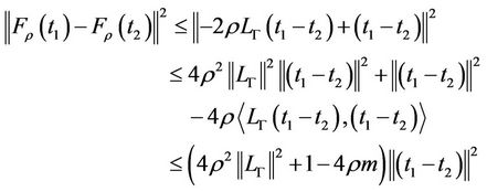
then  is a contractor map, which implies the uniqueness of y* and
 .
.
4.1. Numerical Approach
In this section we describe a numerical scheme which allows the calculation of the initial state gradient between  and
and  on the subregion Γ.
We have seen in the previous section that in order to reconstruct the initial state between  and
and , it is sufficient to solve the Equations (9)-(11), which can be done by the following algorithm of Uzawa type. Let
 , if we choose two functions

and


then we obtain the following algorithm (Table 1).
4.2. Simulation Results
In this section we give a numerical example which
illustrates the efficiency of the previous approach. The results are related to the choice of the subregion, the initial conditions and the sensor location. Let us consider a two-dimensional system defined in  and described by the following parabolic equation

The measurements are given by a pointwise sensor  with b is the location of the sensor and
 . Let
. Let  and
and
the initial gradient to be observed on Γ with g1 and g2 are given by

and

For
and

with

Applying the previous algorithm for , we obtain
“Figures 2 and 3” show that the estimated initial gradient is between  and
and  on the subregion Γ, and show that the sensor located in
  is
is  -gradient strategic on Γ. The estimated initial gradient is obtained with reconstruction error
 .
.
If we take , we obtain “Figure 4”

Figure 2. The first component of the estimated initial gradient, α1(·) and β1(·) on Γ.

Figure 3. The second component of the estimated initial gradient, α2(·) and β2(·) on Γ.
shows that the estimated initial gradient is not between  and
and  on the subregion Γ, which implies that the sensor located in
  is not
  -gradient strategic on Γ.
Remark 4.2
The above results are obtained with pointwise measurement, and one can obtain similar results with zone (internal or boundary) measurement.
5. Conclusions
The problem of  -boundary gradient observability on Γ of parabolic system is considered. The initial state gradient is characterized by two approaches based on regional observability tools in connection with Lagrangian and subdifferential techniques.
Moreover, we have explored à useful numerical algorithm which allows the computation of initial state gradient and which is illustrated by numerical example and simulations. Various questions are still open. The characterization of  -boundary gradient observability by a rank condition as stated for usual gradient observability or regional gradient observability of distributed parameter systems is of great interest. This

Figure 4. The first component of the estimated initial gradient, α1(·) and β1(·) on Γ.
question is under consideration and will be the subject of the future paper.