Convolution Integrals and a Mirror Theorem from Toric Fiber Geometry

Jeff Brown

Baltimore, MD, USA.

DOI: 10.4236/apm.2019.99033                

Abstract

Let E be a toric fibration arising from symplectic reduction of a direct sum of complex line bundles over (almost) Kähler base B. Then each torus-fixed point of the toric manifold fiber defines a section of the fibration. Let L_a be convex line bundles over B, A_a smooth divisors of B arising as the zero loci of generic sections of L_a , and a particular fixed-point section of E. Further assume the {A_a} to be mutually disjoint. The manifold is a new manifold with tautological line bundles over new projective spaces in the geometry, where previously there was a simpler vector bundle in the given local geometry (Section 1.5). Thus, we compute genus-0 Gromov-Witten invariants of in terms of genus-0 Gromov-Witten invariants of B and of {A_a}, the matrix used for the symplectic reduction description of the fiber of the toric fibration E→B, and the restriction maps . The proofs utilize the fixed-point localization technique describing the geometry of and its genus-0 Gromov-Witten theory, as well as the Quantum Lefschetz theorem relating the genus-0 Gromov-Witten theory of A with that of B.

Keywords

Gromov-Witten Invariant, Quantum Cohomology, Fixed-Point Localization, Birational Geometry

1. Introduction

1.1. Formulations

Our main results are formulated in terms of the formal series

${\mathcal{F}}_M\left(t\right)={\displaystyle \underset{n=0}{\overset{\infty }{\sum }}}{\displaystyle \underset{D\in MC}{\sum }}\frac{Q^D}{n\mathrm{<mo>\; !\; </mo>}}{\displaystyle {\int }_{\left[M_{\mathrm{0,}n\mathrm{,}D}\right]}}{\displaystyle \underset{a=1}{\overset{n}{\prod }}}{\displaystyle \underset{k=0}{\overset{\infty }{\sum }}}{\text{ev}}_a^{\mathrm{<mo>\; *\; </mo>}}\left(t_k\right){\psi }_a^k$

called the genus-0 descendant potential of M, where M is respectively $E\parallel \alpha \left(A\right)$ (as in the Abstract), the base of the toric fibration E, or a suitable divisor of the base. The ingredients of the series are defined in the generality of almost-Kähler manifolds M, as follows. The spaces $M_{\mathrm{0,}n\mathrm{,}D}$ are moduli spaces of (equivalence classes of) degree-D stable maps into M of genus-0 (possibly nodal) compact connected holomorphic curves with n marked points. Two such stable maps $\left(f\mathrm{<mo>\; ;\; </mo>}C\mathrm{,}{x}_1\mathrm{,}\cdots \mathrm{,}{x}_n\right)$ and $\left(f^{\prime }\mathrm{<mo>\; ;\; </mo>}{C}^{\prime }\mathrm{,}{x^{\prime }}_1\mathrm{,}\cdots \mathrm{,}{x^{\prime }}_n\right)$ are equivalent if there is a holomorphic automorphism $\varphi \mathrm{<mo>\; :\; </mo>}C\to C^{\prime }$ mapping marked points to marked points and preserving the ordering, such that $f=f^{\prime }\varphi$. For a stable map $\left(f\mathrm{<mo>\; ;\; </mo>}C\mathrm{,}{x}_1\mathrm{,}\cdots \mathrm{,}{x}_n\right)$, the degree-D condition reads $f_{\mathrm{<mo>\; *\; </mo>}}\left(\left[C\right]\right)=D$.

Then, $\left[M_{\mathrm{0,}n\mathrm{,}D}\right]$ denotes the virtual fundamental class of $M_{\mathrm{0,}n\mathrm{,}D}$. The ingredient ${\psi }_a$ is the 1st Chern class of the universal cotangent line bundle over $M_{\mathrm{0,}n\mathrm{,}D}$ whose fiber at a stable map $\left(f\mathrm{<mo>\; ;\; </mo>}C\mathrm{,}{x}_1\mathrm{,}\cdots \mathrm{,}{x}_n\right)$ is the cotangent line along the stable map at the a-th marked point. The maps ${\text{ev}}_a\mathrm{<mo>\; :\; </mo>}{M}_{\mathrm{0,}n\mathrm{,}D}\to M$ evaluate the stable maps at the a-th marked points.

The Mori cone MC of M is the semigroup in $H_2\left(M\mathrm{,}\mathbb{Z}\right)$ generated by classes representable by compact holomorphic curves. Then $Q^D$ is the element in the Novikov ring (the power-series completion of the semigroup algebra of the Mori cone) representing the degree $D\in MC$. Lastly, $t_k\in H^{\mathrm{<mo>\; *\; </mo>}}\left(M\mathrm{,}\mathcal{Q}\right)\mathrm{,}k=\mathrm{0,1,2,}\cdots$ are arbitrary cohomology classes of M with coefficients in a suitable ground ring $\mathcal{Q}$ (for now, the Novikov ring with rational coefficients $\mathbb{Q}$ ).

It is convenient for this purpose to choose a basis $\left\{{\rho }_l\right\}$ of $H^{\mathrm{1,1}}\left(E\parallel \alpha \left(A\right)\mathrm{,}ℂ\right)$, and extend to a basis of $H^2\left(E\parallel \alpha \left(A\right)\mathrm{,}ℂ\right)$. Then, the dual basis can be thought of in terms of a corresponding basis of curve classes, and its extension to $H_2\left(E\parallel \alpha \left(A\right)\mathrm{,}ℂ\right)$. Define Novikov’s variables $Q_l$; these record, for the exponent, the pairing of ${\rho }_l$ on a curve class $\mathcal{D}$. Equivalently, the variable $Q_l$ records the coefficients of the curve classes $\mathcal{D}$ along the dual basis vector to ${\rho }_l$, in the dual basis expansion of $\mathcal{D}\in H_2\left(E\parallel \alpha \left(A\right)\mathrm{,}ℂ\right)$.

1.2. Toric Fibrations

Let $m=\left(m_{ij}\mathrm{<mo>\; |\; </mo>}i=\mathrm{1,}\cdots \mathrm{,}K\mathrm{<mo>\; ;\; </mo>}j=\mathrm{1,}\cdots \mathrm{,}N\right)$ be an integer matrix, and consider the action of $T^K$ on the Hermitian space ${ℂ}^N$ that, for each $j=1,\cdots ,N$, multiplies the coordinate $z_j$ by $\exp \left({\displaystyle {\sum }_{i=1}^K}{m}_{ij}\sqrt{-1}{\theta }_i\right)$. Let $\mu \mathrm{<mo>\; :\; </mo>}{ℂ}^N\to {ℝ}^N$ be the map given by

$\left(z_1\mathrm{,}{z}_2\mathrm{,}\cdots \mathrm{,}{z}_N\right)\to \left({\left|z_1\right|}^2\mathrm{,}{\left|z_2\right|}^2\mathrm{,}\cdots \mathrm{,}{\left|z_N\right|}^2\right)$.

If the moment map $m\circ \mu$ has a regular value $\omega \in {ℝ}^K$, then ${\left(m\circ \mu \right)}^{-1}\left(\omega \right)/T^K$ is a symplectic manifold. This construction is called symplectic reduction. The space ${\left(m\circ \mu \right)}^{-1}\left(\omega \right)/T^K$ is also denoted by ${ℂ}^N\parallel {}_{\omega }T{}^K$, and is equipped with a canonical symplectic form, call it $\omega$, induced by the standard symplectic form on ${ℂ}^N$. All complex line bundles over B may be assumed to have the unitary circle $S^1$ as structure group, as they are induced by pullback from the tautological line bundle over $ℂP^{\infty }$. Given complex line bundles $L_1\mathrm{,}\cdots \mathrm{,}{L}_N$ over B, it follows that $T^N$ is the structure group of the vector bundle $\oplus L_j\to B$. Thus, the fiberwise symplectic reduction of $\oplus L_j$ is well-defined giving the toric fibration $E\to B$. The ith coordinate ${\theta }_i$ on the torus $T^K$ defines a circle bundle over E for which the expression $\sqrt{-1}d{\theta }_i$ defines connection 1-forms in the bundle. Denote by $-P_i$ the first Chern class of the ith circle bundle over E, and $-p_i$ its restriction to a fiber. The $p_1\mathrm{,}\cdots \mathrm{,}{p}_K$ classes are of Hodge $\left(\mathrm{1,1}\right)$ -type by the Fubini-Study construction, though they need not be Kähler classes¹. Let $\gamma$ be any $T^N$ -fixed point of ${\left(m\circ \mu \right)}^{-1}\left(\omega \right)/T^K$, and $p\in {\left(m\circ \mu \right)}^{-1}\left(\omega \right)$ representing the $T^K$ -equivalence class $\gamma$. The orbits $T^{K}p$ and $T^{N}p$ are then identical. It follows that there is some coordinate subspace ${ℂ}^K\subset {ℂ}^N$ with coordinates $z_{j_1}\mathrm{,}\cdots \mathrm{,}{z}_{j_K}$, containing p, such that none of the coordinates $z_{j_1}\left(p\right)\mathrm{,}\cdots \mathrm{,}{z}_{j_K}\left(p\right)$ vanishes. It will be convenient to think of the $T^N$ -fixed strata $\gamma$ of E in terms of the corresponding indices $j_1\mathrm{,}\cdots \mathrm{,}{j}_K$. For each $j=1,\cdots ,N$, the restriction of $U_j={\displaystyle {\sum }_{i=1}^K}{m}_{ij}{P}_i-{\Lambda }_j$ to a fiber is Poincaré dual to the jth coordinate divisor $\left({\left(m\circ \mu \right)}^{-1}\left(\omega \right)\cap \left\{z_j=0\right\}\right)/T^K$. Define $-{\Lambda }_j\mathrm{<mo>\; :\; </mo>}=c_1^T\left(L_j\right)$ for $j=1,\cdots ,N$. The expressions for the pullbacks $P_i^{\gamma }$ in terms of ${\Lambda }_j$ may be summarized by the equations ${\gamma }^{*}{U}_{j_1}=\cdots ={\gamma }^{*}{U}_{j_K}=0$.

Set $T:=T^N$. All bundles introduced thus far are T-equivariant, so their Chern classes may be assumed to take values in the T-equivariant cohomology group $H_T^{\mathrm{<mo>\; *\; </mo>}}\left(E\right)$, or $H_T^{\mathrm{<mo>\; *\; </mo>}}\left({\pi }^{-1}\left(A\right)\right)$, with coefficient ring $H^{\mathrm{<mo>\; *\; </mo>}}\left(BT\mathrm{,}\mathbb{Q}\right)=\mathbb{Q}\left[{\lambda }_1\mathrm{,}\cdots \mathrm{,}{\lambda }_N\right]$.

1.3. The Cone ${\mathcal{L}}_{E\parallel \alpha (A)}$

Associated to the genus-0 Gromov-Witten theory of M is a Lagrangian cone ${\mathcal{L}}_M$ in a symplectic loop space $\left(\mathcal{H}\mathrm{,}\Omega \right)$ [1] [2] [3]. The space $\mathcal{H}={\mathcal{H}}_{+}\oplus {\mathcal{H}}_{-}$ is a module over the ground ring $\mathcal{Q}$. Pending further completions, $\mathcal{H}$ consists of Laurent series in 1/z with coefficients in $H\mathrm{<mo>\; :\; </mo>}=H^{\mathrm{<mo>\; *\; </mo>}}\left(M\mathrm{,}\mathcal{Q}\right)$, completed so that ${\mathcal{H}}_{+}$ consists of elements of $H\left[z\right]$ at each order in Novikov’s variables, and ${\mathcal{H}}_{-}\mathrm{<mo>\; :\; </mo>}=z^{-1}H〚z^{-1}〛$. Identify each $q\left(z\right)={\displaystyle {\sum }_{k=0}}{q}_k{z}^k\in {\mathcal{H}}_{+}$ with the domain variables $t_0\mathrm{,}{t}_1\mathrm{,}{t}_2\mathrm{,}\cdots$ of ${\mathcal{F}}_M$ by the dilaton shift convention $q_k=t_k-{\delta }_{k,1},k=0,\cdots ,\infty$. Take the ring of coefficients for Novikov’s variables to be the (super-commutative) power series ring (with coefficients in the field of fractions $\mathbb{Q}\left(\lambda \right)\mathrm{<mo>\; :\; </mo>}=\mathbb{Q}\left({\lambda }_1\mathrm{,}\cdots \mathrm{,}{\lambda }_N\right)$, in all of our applications) in the formal coordinates along $H^{\mathrm{<mo>\; *\; </mo>}}\left(M\mathrm{,}\mathbb{Q}\right)$, and require the variables $t_0\mathrm{,}{t}_1\mathrm{,}\cdots$ to vanish when Novikov’s variables and formal coordinates along $H^{\mathrm{<mo>\; *\; </mo>}}\left(M\right)$ are all set to zero. This gives a Novikov ring $\mathcal{Q}$ that is consistent with the formula for $I_{E\parallel \alpha \left(A\right)}$ in our Main Theorem.

Let $\left\{{\varphi }_{\mu }\right\}$ be a basis of $H^{\mathrm{<mo>\; *\; </mo>}}\left(M\right)$ and $\left\{{\varphi }^{\mu }\right\}$ the Poincaré-dual basis. Consider the symplectic manifold $T^{\mathrm{<mo>\; *\; </mo>}}{\mathcal{H}}_{+}$ with standard symplectic form ${\displaystyle {\sum }_{k\ge \mathrm{0,}\mu }}d{p}_k^{\mu }\wedge d{q}_{k\mathrm{,}\mu }$. It is symplectomorphic to $\mathcal{H}$ with symplectic form

$\Omega \left(f\mathrm{,}g\right)\mathrm{<mo>\; :\; </mo>}={\text{Res}}_{z=0}{\left(f\left(-z\right)\mathrm{,}g\left(z\right)\right)}_M$,

where ${\left(\cdot \mathrm{,}\cdot \right)}_M$ is the Poincaré pairing.

Let us implement this symplectomorphism via the map

$\left(q\mathrm{,}p\right)\mapsto {\displaystyle \underset{k\ge \mathrm{0,}\mu }{\sum }}{q}_{k\mathrm{,}\mu }{\varphi }^{\mu }{z}^k+{\displaystyle \underset{k\ge \mathrm{0,}\mu }{\sum }}{p}_k^{\mu }{\varphi }_{\mu }{\left(-z\right)}^{-k-1}$.

Consider the graph of the differential of ${\mathcal{F}}_M\left(t\right)$, which is a Lagrangian submanifold in $T^{\mathrm{<mo>\; *\; </mo>}}{\mathcal{H}}_{+}$. From there, we arrive at

$\mathcal{L}\mathrm{<mo>\; :\; </mo>}=\left\{\left(q\mathrm{,}p\right)\mathrm{<mo>\; |\; </mo>}p=d_t{\mathcal{F}}_M\left(t\right)\right\}$

by rigid translation in the direction of the dilaton shift. Thus $\mathcal{L}$ is also a Lagrangian submanifold. Henceforth we consider $\mathcal{L}$ as a submanifold of $\mathcal{H}$. The work of Coates-Givental [1] , establishes that $\mathcal{L}$ is a (Lagrangian) cone as a formal Lagrangian section of $T^{\mathrm{<mo>\; *\; </mo>}}{\mathcal{H}}_{+}$ near $q=-z$; that is,

$T_f\mathcal{L}\cap \mathcal{L}=z{T}_f\mathcal{L}\forall f\in \mathcal{L}$.

In particular, each tangent space is preserved by multiplication by z.

It may be that $\mathcal{L}$ contains (as a limit point) the $\left(q\mathrm{,}p\right)$ -coordinate origin (0, 0), as a special case of Getzler’s [4] , Givental’s [5] solution, and its geometric formulation [1] , of Eguchi-Xiong’s, Dubrovin’s $\left(3g-2\right)$ -jet conjecture, as follows.

The shift of the formal variable $t\left(z\right)$ in the z-(or $\psi$ -) direction appears to be well-understood, so perhaps formality of the geometry (to guarantee convergence of $\mathcal{F}\left(q\right)$ ) in the z-direction need not be assumed. This existence (via convergence) of the “vertex” or the “limiting vertex” of the cone gives an intuitive way to think about the introductory material; however, the author has not studied this convergence sufficiently. In our main theorem, the domain variable $t\left(z\right)$ is consistent with the setting of formal geometry.

The Lagrangian cone $\mathcal{L}$ of the T-equivariant genus-0 Gromov-Witten theory of $E\parallel \alpha \left(A\right)$ lies in the corresponding symplectic loop space $\left(\mathcal{H}\mathrm{,}\Omega \right)$ as above. A point in the cone can be written as

$F\left(-z\mathrm{,}t\right)=-1z+t\left(z\right)+{\displaystyle \underset{n=0}{\overset{\infty }{\sum }}}{\displaystyle \underset{D\in MC}{\sum }}\frac{Q^D}{n\mathrm{<mo>\; !\; </mo>}}{\left({\text{ev}}_1\right)}_{\mathrm{<mo>\; *\; </mo>}}\left[\frac{1}{-z-{\psi }_1}{\displaystyle \underset{i=2}{\overset{n+1}{\prod }}}\left({\text{ev}}_i^{\mathrm{<mo>\; *\; </mo>}}t\right)\left({\psi }_i\right)\right]$,

where ${\left({\text{ev}}_1\right)}_{\mathrm{<mo>\; *\; </mo>}}$ denotes the virtual push-forward by the evaluation map ${\text{ev}}_1\mathrm{<mo>\; :\; </mo>}{\left(E\parallel \alpha \left(A\right)\right)}_{\mathrm{0,}n+\mathrm{1,}D}\to E\parallel \alpha \left(A\right)$, and $t\left(z\right)={\displaystyle {\sum }_{k=0}^{\infty }}{t}_k{z}^k$ is an arbitrary element of ${\mathcal{H}}_{+}$ with coefficients $t_k\in H$. Define the J-function to be the restriction of $F\left(-z\mathrm{,}t\right)$ to values $t_0\in H$ and to $t_k=0$ for all $k>0$. For each $f\in \mathcal{L}$ there is a unique $t\left(f\right)\in H$ such that

$z{T}_f\mathcal{L}\cap \left\{-z+z{\mathcal{H}}_{-}\right\}=J\left(-z\mathrm{,}t\left(f\right)\right)$.

This property of the set of all tangent spaces² of $\mathcal{L}$ to be in 1-1 correspondence with the set H, which is a finite-dimensional $\mathcal{Q}$ -module, is called overruled. For each $t\in H$ and for each open set $U\ni t$, the J-function generates a module over the algebra ${\Gamma }_U\left({\oplus }_{r=0}^{\infty }\left({\otimes }^r{T}_{t}H\right)\otimes \mathbb{Q}\left(z^{-1}\right)\right)$ of differential operators as follows,

$z{\partial }_{a}z{\partial }_{b}J\left(z\mathrm{,}t\right)=z{\partial }_{a{•}_{t}b}J\left(z\mathrm{,}t\right)\mathrm{,}\forall a\mathrm{,}b\in H^{\mathrm{<mo>\; *\; </mo>}}\left(M\mathrm{,}\mathbb{Q}\right)$

where

$a{•}_{t}b\mathrm{<mo>\; :\; </mo>}={\displaystyle \underset{n=0}{\overset{\infty }{\sum }}}{\displaystyle \underset{D\in MC}{\sum }}\frac{Q^D}{n\mathrm{<mo>\; !\; </mo>}}{\varphi }_{\mu }{\displaystyle {\int }_{\left[M_{\mathrm{0,}n+\mathrm{3,}D}\right]}}{\text{ev}}_1^{\mathrm{<mo>\; *\; </mo>}}{\varphi }^{\mu }{\text{ev}}_2^{\mathrm{<mo>\; *\; </mo>}}a{\text{ev}}_3^{\mathrm{<mo>\; *\; </mo>}}b{\displaystyle \underset{i=4}{\overset{n+3}{\prod }}}{\text{ev}}_i^{\mathrm{<mo>\; *\; </mo>}}t$

is the unital, associative, (super-)commutative quantum cup product. Additionally, the J-function satisfies the string and divisor equations:

$z{\partial }_{1_M}J\left(z\mathrm{,}t\right)=J\left(z\mathrm{,}t\right)$,

and

$z{\partial }_{\rho }J\left(z\mathrm{,}t\right)={\displaystyle \underset{D\in MC}{\sum }}{Q}^D\left(\rho +\rho \left(D\right)z\right)J_M^D\left(z\mathrm{,}t\right)\forall \rho \in H^2\left(M\mathrm{,}\mathbb{Q}\right)$

respectively. The graded homogeneity, defined by degrees of formal variables, makes the quantum cup product a degree 0 operation, the J-function graded homogeneous of degree 1, and z of degree 1.

1.4. Twisted Lagrangian Cones

The forgetful maps $f{t}_{n+1}\mathrm{<mo>\; :\; </mo>}{M}_{\mathrm{0,}n+\mathrm{1,}D}\to M_{\mathrm{0,}n\mathrm{,}D}$ induce the K-theoretic push-forward maps ${\left(f{t}_{n+1}\right)}_{\mathrm{<mo>\; *\; </mo>}}\mathrm{<mo>\; :\; </mo>}K\left(M_{\mathrm{0,}n+\mathrm{1,}D}\right)\to K\left(M_{\mathrm{0,}n\mathrm{,}D}\right)$. Let $\mathcal{V}$ be a complex vector bundle over M. The evaluation maps ${\text{ev}}_{n+1}\mathrm{<mo>\; :\; </mo>}{M}_{\mathrm{0,}n+\mathrm{1,}D}\to M$ induce the (virtual-) bundles ${\text{ev}}_{n+1}^{\mathrm{<mo>\; *\; </mo>}}\mathcal{V}$, in terms of which the (virtual-) virtual bundles

${\mathcal{V}}_{\mathrm{0,}n\mathrm{,}D}\mathrm{<mo>\; :\; </mo>}={\left(f{t}_{n+1}\right)}_{\mathrm{<mo>\; *\; </mo>}}{\text{ev}}_{n+1}^{\mathrm{<mo>\; *\; </mo>}}\mathcal{V}\in K\left(M_{\mathrm{0,}n\mathrm{,}D}\right)$

are defined. The fiber of ${\mathcal{V}}_{\mathrm{0,}n\mathrm{,}D}$ over a stable map $\left(f\mathrm{<mo>\; ;\; </mo>}\Sigma \mathrm{,}p\left(\Sigma \right)\right)$ is

$H^0\left(\Sigma \mathrm{,}{f}^{\mathrm{<mo>\; *\; </mo>}}\mathcal{V}\right)\ominus H^1\left(\Sigma \mathrm{,}{f}^{\mathrm{<mo>\; *\; </mo>}}\mathcal{V}\right)$.

Given a characteristic class $c(\cdot )$, define the twisted Poincaré pairing ${\left(a\mathrm{,}b\right)}_{c(\cdot ),\mathcal{V}}\mathrm{<mo>\; :\; </mo>}={\left(a\mathrm{,}c\left(\mathcal{V}\right)b\right)}_M$.

A point in the $\left(c(\cdot ),\mathcal{V}\right)$ -twisted cone can be written as

$F_{c(\cdot ),\mathcal{V}}\left(-z\mathrm{,}t\right)=-1z+t\left(z\right)+{\displaystyle \underset{n\mathrm{,}D}{\sum }}\frac{Q^D}{n\mathrm{<mo>\; !\; </mo>}}{\left({\text{ev}}_{\text{1}}\right)}_{\mathrm{<mo>\; *\; </mo>}}\left[c\left({\mathcal{V}}_{\mathrm{0,}n+\mathrm{1,}D}\right)\frac{1}{-z-{\psi }_1}{\displaystyle \underset{i=2}{\overset{n+1}{\prod }}}\left({\text{ev}}_i^{\mathrm{<mo>\; *\; </mo>}}t\right)\left({\psi }_i\right)\right]$.

The overruled Lagrangian cone ${\mathcal{L}}_{c(\cdot )\mathrm{,}\mathcal{V}}$ in the $\left(c(\cdot ),\mathcal{V}\right)$ -twisted genus-0 Gromov-Witten theory of M lies in the symplectic loop space $\left({\mathcal{H}}^{c(\cdot ),\mathcal{V}}\mathrm{,}{\Omega }_{c(\cdot ),\mathcal{V}}\right)$, where $t\left(z\right)={\displaystyle {\sum }_{k=0}^{\infty }}{t}_k{z}^k$ is an element of ${\mathcal{H}}_{+}^{c(\cdot ),\mathcal{V}}\mathrm{<mo>\; :\; </mo>}={\left({\mathcal{H}}_M\right)}_{+}$ with arbitrary coefficients $t_k\in H^{c(\cdot ),\mathcal{V}}:=H_M$. The examples we will consider are:

Example 1.4.1. $c(\cdot )=Euler(\cdot )$, and $\mathcal{V}$ is a convex line bundle; i.e., $H^1\left(\Sigma \mathrm{,}{f}^{\mathrm{<mo>\; *\; </mo>}}\mathcal{V}\right)=0$; or equivalently, $f^{\mathrm{<mo>\; *\; </mo>}}{c}_1\left(\mathcal{V}\right)\left(\Sigma \right)\ge -1$ for all genus-0 stable maps $\left(f\mathrm{<mo>\; ;\; </mo>}\Sigma \mathrm{,}p\left(\Sigma \right)\right)$ to M.

Example 1.4.2. $c(\cdot )=Eule{r}_T^{-1}(\cdot )$, and $\mathcal{V}$ is a complex vector bundle with a hamiltonian T-action that decomposes $\mathcal{V}$ into a direct sum of complex line bundles, each of which carries a non-trivial T-action.

1.5. Torus Action on $E\parallel \alpha (A)$

The manifold $E\parallel \alpha \left(A\right)$ may be described as the result of surgery on E, along the divisor $\alpha \left(A\right)$ of the T-fixed section $\alpha \subset E$, as we now recall. The notation $E\parallel \alpha \left(A\right)$, and $\tilde{\pi }\mathrm{<mo>\; :\; </mo>}E\parallel \alpha \left(A\right)\to E$ recall the detailed local geometry near the exceptional divisor ${\pi }^{-1}\left(A\right)\simeq i_A^{\mathrm{<mo>\; *\; </mo>}}{N}_{\alpha \left(A\right)}E\parallel {ℂ}^{\mathrm{<mo>\; *\; </mo>}}$. Define a map from a tubular neighborhood of the $O\left(-1\right)$ bundle over the projective space bundle ${\pi }^{-1}\left(A\right)\simeq i_{\alpha \left(A\right)}^{\mathrm{<mo>\; *\; </mo>}}{N}_{\alpha \left(A\right)}E\parallel {ℂ}^{\mathrm{<mo>\; *\; </mo>}}$ over $\alpha \left(A\right)$ to a tubular neighborhood of $N_{\alpha \left(A\right)}E\simeq i_A^{\mathrm{<mo>\; *\; </mo>}}L\oplus i_A^{\mathrm{<mo>\; *\; </mo>}}{N}_{\alpha }E$ over $\alpha \left(A\right)$ as follows. Fiberwise, it is described by the projection map $\tilde{\pi }$

$\begin{array}{l}\left\{\left(v\mathrm{,}\mathcal{l}\right)\in {ℂ}^{N-K+1}\times ℂP^{N-K}\mathrm{<mo>\; :\; </mo>}\mathcal{l}\text{alinein}{ℂ}^{N-K+1}\text{throughtheorigin;}v\in \mathcal{l}\right\}\\ \to {ℂ}^{N-K+1}\mathrm{,}\left(v\mathrm{,}\mathcal{l}\right)\mapsto v.\end{array}$

This construction holds in the generality³ of complex manifolds and submanifolds, respectively, where $N-K+1=di{m}_{ℂ}{N}_{\alpha \left(A\right)}E$ is replaced by $di{m}_{ℂ}$ (normal bundle to the submanifold within the ambient manifold). The map $\tilde{\pi }$ collapses the projective space fibers $0\times ℂP^{N-K}$ fiberwise over $\alpha \left(A\right)$. The map $\tilde{\pi }$ is the identity map away from the points $\left(\mathrm{0,}\mathcal{l}\right)$ above, and thus extends over the entire gluing space $E\parallel \alpha \left(A\right)$. This map identifies T-equivariantly the complements of the 0-sections of the total spaces of the preceding two vector bundles. Remove a tubular neighborhood of $N_{\alpha \left(A\right)}E$ from E, and replace it by a tubular neighborhood of the $O\left(-1\right)$ bundle over ${\pi }^{-1}\left(A\right)\simeq i_A^{\mathrm{<mo>\; *\; </mo>}}{N}_{\alpha \left(A\right)}E\parallel {ℂ}^{\mathrm{<mo>\; *\; </mo>}}$.

We will call the resulting manifold the projective-space (surgery, gluing, quotient) of E along $\alpha \left(A\right)$, the $N_{\alpha \left(A\right)}E\parallel {ℂ}^{\mathrm{<mo>\; *\; </mo>}}$ quotient-space of E along $\alpha \left(A\right)$, the $\left(i_A^{\mathrm{<mo>\; *\; </mo>}}L\oplus i_A^{\mathrm{<mo>\; *\; </mo>}}{N}_{\alpha }E\right)\parallel {ℂ}^{\mathrm{<mo>\; *\; </mo>}}$ quotient-space of E along $\alpha \left(A\right)$ (Section 2.1), the $\parallel {ℂ}^{\mathrm{<mo>\; *\; </mo>}}$ surgery-space of E along (or normal to) $\alpha \left(A\right)$. Henceforth, we denote this by $E\parallel \alpha \left(A\right)$, for simplicity of notation.

1.6. Simplification: Toric Manifold

Let X be a compact symplectic toric manifold and let $T\subset {\left({ℂ}^{\mathrm{<mo>\; *\; </mo>}}\right)}^{di{m}_{ℂ}X}$ be the maximal unitary torus, and let Y be a T-invariant submanifold of X. Then $X\parallel Y$ is again a toric manifold. As explained in Section 1.5, though not in the generality needed here, the action of T on X induces an action of T on $X\parallel Y$. Thus, we may study T-equivariant genus-0 Gromov-Witten invariants of $X\parallel Y$, the ${ℂ}^{\mathrm{<mo>\; *\; </mo>}}$ -quotient of X along (or normal to) Y directly, using fixed-point localization. All faces of the moment polytope of Y are faces of the moment polytope of X. The moment polytope of $X\parallel Y$ admits a canonical inclusion into the moment polytope of X, for which all faces of the moment polytope of $X\parallel Y\backslash {\pi }^{-1}\left(Y\right)\simeq X\parallel Y\backslash \left(N_{Y}X\right)\parallel {ℂ}^{\mathrm{<mo>\; *\; </mo>}}\simeq X\parallel Y\backslash \mathbb{P}\left(N_{Y}X\right)$ are contained in faces of the corresponding same dimension of the moment polytope of X. Let $v_1\mathrm{,}\cdots \mathrm{,}{v}_m$ be the primitive integer normal vectors to the codimension one faces of the moment polytope of a toric manifold. Let $m_1\mathrm{,}\cdots \mathrm{,}{m}_K$ be a basis of the $\mathbb{Q}$ -vector space

$\left\{\left(a_1,\cdots ,a_m\right)|{\displaystyle \underset{i=1}{\overset{m}{\sum }}}{a}_i{v}_i=0\right\},$

consisting of primitive integer vectors. The toric manifold is then recovered from symplectic reduction referred to the matrix $m$, whose row vectors are $m_1\mathrm{,}\cdots \mathrm{,}{m}_K$. By a mirror theorem of Givental [6] and its extensions [7] , a particular family of points on the Lagrangian cone of the genus-0 Gromov-Witten theory of a toric manifold is given by an explicit formula⁴ in terms of $m_1\mathrm{,}\cdots \mathrm{,}{m}_K$,

$I_X\left(t\mathrm{,}z\right)\mathrm{<mo>\; :\; </mo>}=z{\text{e}}^{Pt/z}{\displaystyle \underset{d\in MC\left(X\right)}{\sum }}{\left(q{\text{e}}^t\right)}^d\frac{1}{{\displaystyle {\prod }_{m=1}^{U_j\left(d\right)}\left(U_j+mz\right)}}\mathrm{.}$

This project has its roots in the following instructive example. Let E be the total space of the projective bundle

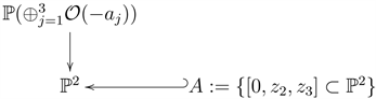
described by symplectic reduction with respect to the matrix

$m_X=\left(\begin{array}{cccccc}1& 1& 1& -a_1& -a_2& -a_3\\ 0& 0& 0& 1& 1& 1\end{array}\right)\mathrm{.}$

Let $\left[\mathrm{0,0,1}\right]$ be the section of E that maps each point $x\in {\mathbb{P}}^2$ to the point $\left[\mathrm{0,0,1}\right]$ in the fiber over x. When X is the toric bundle E and Y is $\left[\mathrm{0,0,1}\right]\left(A\right)$ then a calculation gives

$m_{\left(X\parallel Y\right)}=\left(\begin{array}{ccccccc}1& 1& 1& -a_1& -a_2& -a_3& 0\\ 0& 0& 0& 1& 1& 1& 0\\ 1& 0& 0& 1& 1& 0& -1\end{array}\right)\mathrm{.}$

In particular,

$c_1\left(T\left(X\parallel Y\right)\right)=“\text{thepullbackof}{c}_1\left(TX\right)”+2P_3\mathrm{.}$

This example provides a reference point for navigating the project. The matrix may be computed using Appendix A in [8] , which is itself a summary of literature [9] [10] [11] [12] on moment maps and aspects of toric manifolds. Namely, in the momentum polyhedron of a toric manifold, the 1-dim edge vectors leaving a vertex at a T-fixed point $\gamma$ are positive multiples of the elements of the set ${\left\{{\gamma }^{\mathrm{<mo>\; *\; </mo>}}{U}_j\right\}}_{j\notin \gamma }$. These latter are the weights of the T-action on the normal bundle to $\gamma$ in the toric manifold.

Apply this first to the original projective bundle $X=E$. Then compute the weights of the T-action on the normal bundles in $X\parallel Y$ to the T-fixed points of the exceptional divisor. Finally, compute the normals to the codimension one faces of the momentum polyhedron of $X\parallel Y$. A basis of linear relations among them is given by the rows of the matrix.

However, in fact, our main theorem arises as a generalization of this example. Here we are using the toric mirror theorems [6] [7] [8] as a guide to the structure of genus-0 Gromov-Witten invariants more generally (following the initial proposals of A. Elezi and A. Givental). Elezi’s work focused on projective bundles [13]. In [14] , Givental proposed a toric bundles generalization of Elezi’s approach using toric mirror integral representations [6] [7]. This is an ingredient in [8] and in the present work.

1.7. Organization of the Text

We recall in Section 2.2 the Atiyah-Bott fixed-point localization Theorem which implies, in particular, that any element of $H_T^{\mathrm{<mo>\; *\; </mo>}}\left(E\parallel \alpha \left(A\right)\right)$ is uniquely determined by its restrictions to the T-fixed strata $\epsilon$ of $E\parallel \alpha \left(A\right)$. Points $F\left(z\right)$ on the overruled Lagrangian cone of the genus-0 T-equivariant Gromov-Witten theory of $E\parallel \alpha \left(A\right)$ are certain H-valued formal functions, which we study in terms of their restrictions $\left\{{\epsilon }^{\mathrm{<mo>\; *\; </mo>}}F\left(z\right)\right\}$. As we recall [8] in Section 5, the ${\mathcal{H}}_{-}$ projection of each of the restrictions ${\epsilon }^{\mathrm{<mo>\; *\; </mo>}}F\left(z\right)$ consists of two types of terms. Namely, there are terms ii) that form simple poles expanded as $z^{-1}$ series about non-zero $H_T^{\mathrm{<mo>\; *\; </mo>}}\left(B\right)$ -values of z. The remaining terms i) are polynomial in $z^{-1}$ at any given order in formal variables $t\mathrm{,}\tilde{t}\mathrm{,}q\mathrm{,}\tilde{q}\mathrm{,}\tau \mathrm{,}Q$. The organising principle of the text, formulated as Theorem 2, characterizes the Lagrangian cone of the genus-0 T-equivariant Gromov-Witten theory of $E\parallel \alpha \left(A\right)$ in terms of two conditions i) ii) on $\left\{{\epsilon }^{\mathrm{<mo>\; *\; </mo>}}F\left(z\right)\right\}$. The condition ii) says that the residues of ${\epsilon }^{\mathrm{<mo>\; *\; </mo>}}F$ at its simple poles at non-zero values of z are governed recursively with respect to $\left\{{\epsilon }^{\mathrm{<mo>\; *\; </mo>}}F\left(z\right)\right\}$. The condition i) describes the remaining poles at $z=0$ in terms of a certain twisted Lagrangian cone of the stratum $\epsilon$. The Main Theorem gives a family of points $I_{E\parallel \alpha \left(A\right)}$ whose restrictions satisfy the conditions of Theorem 2.

In Section 6 we verify condition ii) for the restrictions $\left\{{\epsilon }^{\mathrm{<mo>\; *\; </mo>}}{I}_{E\parallel \alpha \left(A\right)}\right\}$ directly, using their defining formulae. In Section 7, we verify condition i) using transformation laws [1] of Lagrangian cones with respect to the twisting construction from Section 1.4 and example 1.8 (expanding simple poles at non-zero values of z in non-negative powers of z). A new aspect of the present work relative to toric bundles is that ii) relates the series $\left\{{\epsilon }^{\mathrm{<mo>\; *\; </mo>}}F\left(z\right)\right\}$ that, according to condition i), lie in Lagrangian cones derived from genus-0 Gromov-Witten invariants of B and of $A_a$, respectively. The Quantum Lefschetz Theorem relates the Lagrangian cone associated to the genus-0 Gromov-Witten theory of A with that of B. If the push-forward $i_{A_a}{}_{\mathrm{<mo>\; *\; </mo>}}\mathrm{<mo>\; :\; </mo>}{H}_2\left(A_a\mathrm{,}\mathbb{Z}\right)\to H_2\left(B\mathrm{,}\mathbb{Z}\right)$ does not identify the Mori cone of $A_a$ with that of B, the opposite relation describing the Lagrangian cone of B in terms of that of $A_a$ is realised algebraically by the Birkhoff factorization procedure and dividing by powers of z. Division by z does not preserve the Lagrangian cone, so we must then clear denominators on both sides. For each $D\in MC\left(B\right)$, denote the greatest power of z that we divide by up to order $Q^D$ in this process by $h{t}_A\left(D\right)$. We work out an example where A is a smooth quintic 3-fold.

It suffices without loss of generality to assume that $\left\{A_a\right\}$ is a single connected manifold A, as regards most aspects of the project. In case there is a subtlety, we address it as it arises.

A key result to keep in mind while reading the paper is the Proposition in Section 2.1, describing the T-equivariant normal bundles to the T-fixed sections of the exceptional divisor. The Proposition is used for both the Atiyah-Bott fixed-point localization theorem for $H_T^{\mathrm{<mo>\; *\; </mo>}}\left(E\parallel \alpha \left(A\right)\right)$ in Section 2.2, and for stating the twisting construction in genus-0 Gromov-Witten theory in Section 7.1 for ${\left(\alpha \mathrm{,}{j}_{+}\right)}^{\mathrm{<mo>\; *\; </mo>}}{I}_{E\parallel \alpha \left(A\right)}$.

1.8. T-Fixed Strata of $E\parallel \alpha (A)$

Recall that L gives rise to $A\subset B$ as the zero locus of a generic section. The tautological line bundle with fiber $\mathcal{l}$, i.e. the $\mathcal{O}\left(-1\right)$ bundle, over the exceptional divisor ${\pi }^{-1}\left(A\right)\simeq \mathbb{P}\left(N_{\alpha \left(A\right)}E\right)\simeq \left(i_A^{\mathrm{<mo>\; *\; </mo>}}L\oplus i_A^{\mathrm{<mo>\; *\; </mo>}}{N}_{\alpha }E\right)\parallel {ℂ}^{\mathrm{<mo>\; *\; </mo>}}$ is central to the results.

The T-action on $E\parallel \alpha \left(A\right)$ induces a T-action on the moduli spaces of stable maps to $E\parallel \alpha \left(A\right)$, which in turn induces a T-action on the universal cotangent line bundles at each of the marked points. For a given T-fixed stratum $\epsilon$ of $E\parallel \alpha \left(A\right)$ and a line bundle $\mathcal{V}\to \epsilon$ with a fiberwise T-action, we refer to the class $Eule{r}_T\left(\mathcal{V}\right)\in H_T^2\left(\epsilon \mathrm{,}\mathbb{Q}\right)\simeq H^2\left(BT\mathrm{,}\mathbb{Q}\right)\oplus H^2\left(\epsilon \mathrm{,}\mathbb{Q}\right)$ as the T-weight of $\mathcal{V}$ at $\epsilon$. The T-fixed strata of $E\parallel \alpha \left(A\right)$ are in comparison with those of E as follows. The stratum $\alpha \left(B\right)$ of E is replaced by $\alpha \left(B\right)\parallel \alpha \left(A\right)=\mathrm{<mo>\; :\; </mo>}\tilde{\alpha }$, which is canonically diffeomorphic to $\alpha \left(B\right)$. Let $\epsilon$ take on the values $\left(\alpha \mathrm{,}\left[\mathrm{1,}\stackrel{\to }{0}\right]\right)$ as a substratum of $\tilde{\alpha }$, as well as $\epsilon =\tilde{\alpha }\left(B\right)\backslash \left(\alpha \mathrm{,}\left[\mathrm{1,}\stackrel{\to }{0}\right]\right)$.

Example 1.8. If $\epsilon$ is a T-fixed stratum in the complement of the exceptional divisor, then take $M=B\simeq \epsilon$ in Example 1.4.2. If $\epsilon$ is a T-fixed stratum in the exceptional divisor, then take $M=A\simeq \epsilon$ in Example 1.4.2. In either case, set $\mathcal{V}=N_{\epsilon }\left(E\parallel \alpha \left(A\right)\right)$ in Example 1.4.2 and also define ${\mathcal{N}}^{\epsilon }\mathrm{<mo>\; :\; </mo>}=N_{\epsilon }\left(E\parallel \alpha \left(A\right)\right)$.

Finally, set ${\mathcal{N}}^{\left(\alpha \mathrm{,}\left[\mathrm{1,}\stackrel{\to }{0}\right]\right)}=i_{\left(\alpha \mathrm{,}\left[\mathrm{1,}\stackrel{\to }{0}\right]\right)}^{\mathrm{<mo>\; *\; </mo>}}{\mathcal{N}}^{\tilde{\alpha }}\simeq i_A^{\mathrm{<mo>\; *\; </mo>}}{\mathcal{N}}^{\tilde{\alpha }}$.

For each T-fixed section $\gamma \ne \alpha$ of E, the strata $\gamma \left(B\right)$ of E is canonically a stratum of $E\parallel \alpha \left(A\right)$ that we also denote by $\gamma \left(B\right)$. Lastly, there are T-fixed strata of $E\parallel \alpha \left(A\right)$ that have no counterpart in E. Namely, each T-equivariant line bundle summand of $N_{\alpha \left(A\right)}E\simeq \left(i_A^{\mathrm{<mo>\; *\; </mo>}}L\oplus i_A^{\mathrm{<mo>\; *\; </mo>}}{N}_{\alpha }E\right)$ gives rise to a T-fixed section over A in the exceptional divisor.

In the case $\epsilon =\left(\alpha \mathrm{,}\left[\mathrm{1,}\stackrel{\to }{0}\right]\right)$, ${\epsilon }^{\mathrm{<mo>\; *\; </mo>}}$ will denote (Section 2.1 for the definition) $Im\left(c_1\left(L\right)\cdot \right)/c_1\left(L\right)\subset {\tilde{\alpha }}^{\mathrm{<mo>\; *\; </mo>}}$ rather than the pullback to $H^{\mathrm{<mo>\; *\; </mo>}}\left(A\right)$ (which is modded out as in Section 2.1). Thus, ${\epsilon }^{\mathrm{<mo>\; *\; </mo>}}$ is given a new definition in this case. Let also $\gamma$ take the value $\gamma =Ker\left(c_1\left(L\right)\cdot \right)\subset {\tilde{\alpha }}^{\mathrm{<mo>\; *\; </mo>}}$.

In particular (Section 2.1), the summand $i_A^{\mathrm{<mo>\; *\; </mo>}}L$ gives rise to a section

$\left[\mathrm{1,0,}\cdots \mathrm{,0}\right]\mathrm{<mo>\; :\; </mo>}=\left(N_{\alpha \left(A\right)}\alpha \left(B\right)\oplus 0\right)\parallel {ℂ}^{\mathrm{<mo>\; *\; </mo>}}\simeq \mathbb{P}\left(N_{\alpha \left(A\right)}\alpha \left(B\right)\right)\subset \tilde{\alpha }$

over A in the total space of the exceptional divisor. The T-fixed set $\left(\alpha \mathrm{,}\left[\mathrm{1,}\stackrel{\to }{0}\right]\right)$ is only a proper subset of the T-fixed stratum $\tilde{\alpha }$. Thus we must check the conditions 1.a) and 2.aa) for the projections to $Ker\left(c_1\left(L\right)\cdot \right)\mathrm{,}Im\left(c_1\left(L\right)\cdot \right)/c_1\left(L\right)\subset {\tilde{\alpha }}^{\mathrm{<mo>\; *\; </mo>}}$ (see Section 7.3 for the integral asymptotics of $\tilde{\alpha }$ ), and not for ${\left(\alpha \mathrm{,}\left[\mathrm{1,}\stackrel{\to }{0}\right]\right)}^{\mathrm{<mo>\; *\; </mo>}}$, for the series $I_{E\parallel \alpha \left(A\right)}$.

From now on let the symbol $\gamma$ stand for the T-fixed strata denoted $\gamma$ above, or for the “substrata” $Ker\left(c_1\left(L\right)\cdot \right)\subset {\tilde{\alpha }}^{\mathrm{<mo>\; *\; </mo>}}$ of $\tilde{\alpha }$. Let us denote the situation of a torus fixed point $\beta$ connected to $\alpha$ by a 1-dimensional edge of the momentum polyhedron of a fiber of E, by $\beta ~\alpha$. In this case $\left|\alpha \cup \beta \right|=K+1$, $\left|\alpha \cap \beta \right|=K-1$, and ${ℂ}^{\alpha \cup \beta }\parallel T^K=\mathrm{<mo>\; :\; </mo>}ℂP_{\alpha \mathrm{,}\beta }^1$. Let $j_{-}\left(\alpha \mathrm{,}\beta \right)$ be the coordinate from $\alpha \backslash \alpha \cap \beta$ and $j_{+}\left(\alpha \mathrm{,}\beta \right)$ the coordinate from $\beta \backslash \alpha \cap \beta$. Similarly, we have the notation $\alpha \left(\beta \mathrm{,}{j}_{-}\right)$ and $\beta \left(\alpha \mathrm{,}{j}_{+}\right)$. In the next section, we enhance this description of the T-fixed points of E to a description of the T-fixed points of $E\parallel \alpha \left(A\right)$.

2. Geometry of $E\parallel \alpha (A)$

2.1. Geometric Preliminaries and Decomposition of Cohomology

The action of T on E decomposes $i_{\alpha \left(A\right)}^{\mathrm{<mo>\; *\; </mo>}}TE/T\alpha \left(A\right)$ into a direct sum of 1-dimensional eigenspaces,

$N_{\alpha \left(A\right)}E=i_{\alpha \left(A\right)}^{\mathrm{<mo>\; *\; </mo>}}TE/T\alpha \left(A\right)\simeq i_{\alpha \left(A\right)}^{\mathrm{<mo>\; *\; </mo>}}T\alpha \left(B\right)/T\alpha \left(A\right)\oplus i_{\alpha \left(A\right)}^{\mathrm{<mo>\; *\; </mo>}}{N}_{\alpha }E\simeq i_A^{\mathrm{<mo>\; *\; </mo>}}L\oplus i_{\alpha \left(A\right)}^{\mathrm{<mo>\; *\; </mo>}}{N}_{\alpha }E\mathrm{.}$

Let $j{j}_{+}$ be an ordering index of these eigenspaces, where the index value $j{j}_{+}=\left[\mathrm{1,}\stackrel{\to }{0}\right]$ corresponds to the bundle $i_A^{\mathrm{<mo>\; *\; </mo>}}L$, and $j{j}_{+}=j_{+}$ indexes the summand of $N_{\alpha }E$ with T-weight ${\alpha }^{\mathrm{<mo>\; *\; </mo>}}{U}_{j_{+}}$. Denote the T-fixed section of ${\pi }^{-1}\left(A\right)\simeq \left(i_A^{\mathrm{<mo>\; *\; </mo>}}L\oplus i_A^{\mathrm{<mo>\; *\; </mo>}}{N}_{\alpha }E\right)\parallel {ℂ}^{\mathrm{<mo>\; *\; </mo>}}$ corresponding to the index $j{j}_{+}$ by $\left(\alpha \mathrm{,}j{j}_{+}\right)$. In the $l-E\parallel \alpha \left(A\right)$ case, we need to include the index a, for the divisors of B along which we replace the geometry of E by the $E\parallel \alpha \left(A_a\right)$ geometry. The strata $\left(\alpha \mathrm{,}{j}_{+}\right)$ is connected to the strata $\beta \left(\alpha \mathrm{,}{j}_{+}\right)$ by the T-invariant edges $ℂP_{\left(\alpha \mathrm{,}{j}_{+}\right)\mathrm{,}\beta }^1$. Denote by ${\chi }_{\epsilon \mathrm{,}{\epsilon }^{\prime }}\in H_T^2\left(\epsilon \right)$ the T-weight of $T_{\epsilon }ℂP_{\epsilon \mathrm{,}{\epsilon }^{\prime }}^1$.

Denote by $\pi \mathrm{<mo>\; :\; </mo>}E\parallel \alpha \left(A\right)\to B$ the composition of $\tilde{\pi }\mathrm{<mo>\; :\; </mo>}E\parallel \alpha \left(A\right)\to E$ with the projection to the base B. It is now mandatory that we introduce the diagram

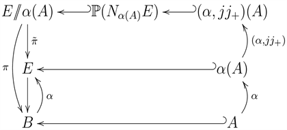
Let $N^{\left(\alpha \mathrm{,}j{j}_{+}\right)}$ be the normal bundle within $E\parallel \alpha \left(A\right)$ to the T-fixed section over A with index $j{j}_{+}$ in $\mathbb{P}\left(N_{\alpha \left(A\right)}E\right)\simeq \left(i_A^{\mathrm{<mo>\; *\; </mo>}}L\oplus i_A^{\mathrm{<mo>\; *\; </mo>}}{N}_{\alpha }E\right)\parallel {ℂ}^{\mathrm{<mo>\; *\; </mo>}}$.

Proposition. The action of T on $E\parallel \alpha \left(A\right)$ decomposes $N^{\left(\alpha \mathrm{,}j{j}_{+}\right)}$ into a direct sum of T-equivariant line bundles, whose T-equivariant Euler classes are the elements of the set

$\begin{array}{l}\text{if}j{j}_{+}=j_{+}\mathrm{<mo>\; :\; </mo>}\\ {\left\{-{\alpha }^{\mathrm{<mo>\; *\; </mo>}}{U}_{j{j}_{+}}+{\alpha }^{\mathrm{<mo>\; *\; </mo>}}{U}_j\right\}}_{j\ne j{j}_{+}\mathrm{,}\notin \alpha }\cup \left\{-{\alpha }^{\mathrm{<mo>\; *\; </mo>}}{U}_{j{j}_{+}}+i_A^{\mathrm{<mo>\; *\; </mo>}}{c}_1\left(L\right)\right\}\cup \left\{{\alpha }^{\mathrm{<mo>\; *\; </mo>}}{U}_{j{j}_{+}}\right\}\mathrm{,}\\ \text{if}j{j}_{+}=\left[\mathrm{1,}\stackrel{\to }{0}\right]\mathrm{<mo>\; :\; </mo>}\\ {\left\{-i_A^{\mathrm{<mo>\; *\; </mo>}}{c}_1\left(L\right)+{\alpha }^{\mathrm{<mo>\; *\; </mo>}}{U}_j\right\}}_{j\notin \alpha }\cup \left\{i_A^{\mathrm{<mo>\; *\; </mo>}}{c}_1\left(L\right)\right\}\mathrm{.}\end{array}$

Let us now turn attention to the restriction map $H^{\mathrm{<mo>\; *\; </mo>}}\left(E\parallel \alpha \left(A\right)\right)\to H^{\mathrm{<mo>\; *\; </mo>}}\left({\pi }^{-1}\left(A\right)\right)$. Denote $\tilde{P}$ the T-equivariant Euler class of the ${\mathcal{O}}_T\left(1\right)$ bundle on the exceptional divisor. By the Lerray-Serre theorem,

$H^{\mathrm{<mo>\; *\; </mo>}}\left({\pi }^{-1}\left(A\right)\right)\simeq H^{\mathrm{<mo>\; *\; </mo>}}\left(A\right)\left[\tilde{P}\right]\mathrm{.}$

In the following, we extend the definition of $\tilde{P}$ to the entire $E\parallel \alpha \left(A\right)$. With this interpretation of $\tilde{P}$, recall the isomorphism of vector spaces [15]

$H^{\mathrm{<mo>\; *\; </mo>}}\left(E\parallel \alpha \left(A\right)\right)\simeq H^{\mathrm{<mo>\; *\; </mo>}}\left(E\right)\oplus \left(H^{\mathrm{<mo>\; *\; </mo>}}\left({\pi }^{-1}\left(A\right)\right)/H^{\mathrm{<mo>\; *\; </mo>}}\left(A\right)\right)\mathrm{,}$

where the quotient is an additive quotient and $H^{\mathrm{<mo>\; *\; </mo>}}\left(E\right)\simeq Im\left({\tilde{\pi }}^{\mathrm{<mo>\; *\; </mo>}}\right)$. On the other hand, $H^{\mathrm{<mo>\; *\; </mo>}}\left(E\right)\simeq H^{\mathrm{<mo>\; *\; </mo>}}\left(B\right)\left[P_1\mathrm{,}\cdots \mathrm{,}{P}_K\right]$. The restriction of $P_i$ to the exceptional divisor is ${\tilde{\pi }}^{\mathrm{<mo>\; *\; </mo>}}{i}_{\alpha \left(A\right)}^{\mathrm{<mo>\; *\; </mo>}}{P}_i$, which restricts to $i_{\alpha \left(A\right)}^{\mathrm{<mo>\; *\; </mo>}}{P}_i$ to $\left(\alpha \mathrm{,}j{j}_{+}\right)\left(A\right)$.

Let us assume that $Im\left(i_A^{\mathrm{<mo>\; *\; </mo>}}\right)\cap {\left(Im\left(i_A^{\mathrm{<mo>\; *\; </mo>}}\right)\right)}^{\perp }=0$, so that

$H^{\mathrm{<mo>\; *\; </mo>}}\left(A\right)\simeq Im\left(i_A^{\mathrm{<mo>\; *\; </mo>}}\right)\oplus {\left(Im\left(i_A^{\mathrm{<mo>\; *\; </mo>}}\right)\right)}^{\perp }\mathrm{.}$

This holds true in the examples of quintic 3-folds for which the base is projective space. More generally, examples follow from the Lefschetz hyperplane Theorem and the Hard Lefschetz Theorem.

The restriction map $i_A^{\mathrm{<mo>\; *\; </mo>}}\mathrm{<mo>\; :\; </mo>}{H}^{\mathrm{<mo>\; *\; </mo>}}\left(B\right)\to H^{\mathrm{<mo>\; *\; </mo>}}\left(A\right)$ and the Poincaré pairing give the orthogonal projection ${\pi }^{\perp }$ :

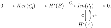
The short exact sequence

$0\to Ker\left(c_1\left(L\right)\cdot \right)\to H^{\mathrm{<mo>\; *\; </mo>}}\left(B\right)\stackrel{c_1\left(L\right)\cdot }{\to }Im\left(c_1\left(L\right)\cdot \right)\to 0$

gives a direct sum decomposition $H^{\mathrm{<mo>\; *\; </mo>}}\left(B\right)\simeq Ker\left(c_1\left(L\right)\cdot \right)\oplus Im\left(c_1\left(L\right)\cdot \right)/c_1\left(L\right)$ with respect to the Poincaré-pairing on $H^{\mathrm{<mo>\; *\; </mo>}}\left(B\right)$.

The result of “division by $c_1\left(L\right)$ ” is only defined at the level of coset representatives of $H^{\mathrm{<mo>\; *\; </mo>}}\left(B\right)/Ker\left(c_1\left(L\right)\cdot \right)$. The choice of a basis of coset representatives from $H^{\mathrm{<mo>\; *\; </mo>}}\left(B\right)$ suffices for integration over $\tilde{\alpha }\left(B\right)$ weighted by $c_1\left(L\right)$, which represents integration over the fundamental class of $\tilde{\alpha }\left(A\right)$. Thus, the subspace $Im\left(c_1\left(L\right)\cdot \right)/c_1\left(L\right)$ represents the span of an arbitrary basis of coset representatives from $H^{\mathrm{<mo>\; *\; </mo>}}\left(B\right)$, and is not uniquely defined. The space $Im\left(c_1\left(L\right)\cdot \right)/c_1\left(L\right)$ can be thought of as $H^{\mathrm{<mo>\; *\; </mo>}}\left(B\right)/Ker\left(c_1\left(L\right)\cdot \right)$.

For the purpose of integrating over fundamental cycles, the pullback $i_A^{\mathrm{<mo>\; *\; </mo>}}\left(b\right)$, $\forall b\in H^{di{m}_{ℝ}B-2}\left(B\right)$, of b to $H^{\mathrm{<mo>\; *\; </mo>}}\left(A\right)$ can be described with respect to $H^{\mathrm{<mo>\; *\; </mo>}}\left(B\right)$ by a multiplicative factor of $c_1\left(L\right)$,

${\displaystyle {\int }_A}{i}_A^{\mathrm{<mo>\; *\; </mo>}}b={\displaystyle {\int }_B}{c}_1\left(L\right)b\mathrm{.}$

Let us now establish that

$Ker\left(i_A^{\mathrm{<mo>\; *\; </mo>}}\right)\subset Ker\left(c_1\left(L\right)\cdot \right)\mathrm{.}$

Both are subsets of $H^{\mathrm{<mo>\; *\; </mo>}}\left(B\right)$. In general, the subspaces can differ only on $H^{di{m}_{ℂ}B}\left(B\right)$, about which the Hodge diamond is symmetric w.r.t. the Lefschetz theorems. The inclusion is clearly an isomorphism when the base is projective space.

Thus, $\forall c\in Ker\left(i_A^{\mathrm{<mo>\; *\; </mo>}}\right)\mathrm{,}\forall b\in H^{\mathrm{<mo>\; *\; </mo>}}\left(B\right)$,

${\displaystyle {\int }_A}{i}_A^{*}\left(cb\right)={\displaystyle {\int }_B}\left(c_1\left(L\right)c\right)b=0.$

Thus, $c_1\left(L\right)c=0$. This gives the inclusion. Finally, taking the quotients of $H^{\mathrm{<mo>\; *\; </mo>}}\left(B\right)$ gives

$Im\left(i_A^{\mathrm{<mo>\; *\; </mo>}}\right)\simeq H^{\mathrm{<mo>\; *\; </mo>}}\left(B\right)/Ker\left(i_A^{\mathrm{<mo>\; *\; </mo>}}\right)\to H^{\mathrm{<mo>\; *\; </mo>}}\left(B\right)/Ker\left(c_1\left(L\right)\cdot \right)\simeq Im\left(c_1\left(L\right)\cdot \right)/c_1\left(L\right)\mathrm{.}$

Let us assume the map on the LHS is an isomorphism (an equality). This is also assumed as hypotheses for the main theorem (Section 4) and Theorem 2.

The RHS is used in the comparison of projection maps. Then, ${\pi }_{Ker\left(c_1\left(L\right)\cdot \right)}$ and ${\pi }_{Im\left(c_1\left(L\right)\cdot \right)/c_1\left(L\right)}$ extend to $H^{\mathrm{<mo>\; *\; </mo>}}\left(E\parallel \alpha \left(A\right)\right)$ by

${\pi }_{Ker\left(c_1\left(L\right)\cdot \right)}\tilde{P}=\mathrm{0,}$

and

${\tilde{P}}^{\left(\alpha \mathrm{,}\left[\mathrm{1,}\stackrel{\to }{0}\right]\right)}\mathrm{<mo>\; :\; </mo>}={\pi }_{Im\left(c_1\left(L\right)\cdot \right)/c_1\left(L\right)}\tilde{P}=-{\pi }_{Im\left(c_1\left(L\right)\cdot \right)/c_1\left(L\right)}{c}_1\left(L\right)\mathrm{,}$

respectively.

2.2. Fixed-Point Localization

For each $\epsilon \in {\left(E\parallel \alpha \left(A\right)\right)}^T$, the action of T on $E\parallel \alpha \left(A\right)$ decomposes $N_{\epsilon }E\parallel \alpha \left(A\right)$ into a direct sum of 1-dimensional eigenspaces. Define $N^{\epsilon }$ as in Example 1.8. Let $U_{A\mathrm{,}jj}\in H_T^2\left({\pi }^{-1}\left(A\right)\right)$ be the classes that restrict to the T-equivariant Poincaré duals of the torus-invariant divisors in the fibers of the exceptional divisor ${\pi }^{-1}\left(A\right)\simeq \left(i_A^{\mathrm{<mo>\; *\; </mo>}}L\oplus i_A^{\mathrm{<mo>\; *\; </mo>}}{N}_{\alpha }E\right)\parallel {ℂ}^{\mathrm{<mo>\; *\; </mo>}}$ :

$U_{A\mathrm{,}jj}=\{\begin{array}{ll}\tilde{P}+i_{\alpha \left(A\right)}^{\mathrm{<mo>\; *\; </mo>}}{\alpha }^{\mathrm{<mo>\; *\; </mo>}}{U}_j,\hfill & jj=j\notin \alpha \hfill \\ \tilde{P}+i_{\alpha \left(A\right)}^{\mathrm{<mo>\; *\; </mo>}}{c}_1\left(L\right),\hfill & jj=\left[\mathrm{1,}\stackrel{\to }{0}\right]\hfill \end{array}\in H_T^2\left(\left[\mathrm{1,}\stackrel{\to }{0}\right]A\right)\mathrm{.}$

The Atiyah-Bott Theorem says that the pairing of a class $f\in H_T\left(E\parallel \alpha \left(A\right)\right)$ against the fundamental class of $E\parallel \alpha \left(A\right)$ is given by

$\begin{array}{c}{\displaystyle {\int }_{E\parallel \alpha \left(A\right)}}f={\displaystyle \underset{\gamma \ne \tilde{\alpha }}{\sum }}{\displaystyle {\int }_{\gamma \left(B\right)}}{\text{Res}}_{U_{j_1}=\cdots =U_{j_K}=0}\frac{f\text{d}{P}_1\wedge \cdots \wedge \text{d}{P}_K}{U_1\cdots U_n}det\left(\text{d}U/\text{d}P\right)\\ +{\displaystyle {\int }_{\tilde{\alpha }\left(B\right)}}{\text{Res}}_{U_{j_1}=\cdots =U_{j_K}=0}\frac{f\text{d}{P}_1\wedge \cdots \wedge \text{d}{P}_K}{\left({\displaystyle {\prod }_{j\in \alpha }{U}_j}\right)\left({\displaystyle {\prod }_{j\notin \alpha }{U}_j}+\tilde{P}\right)}det\left(\text{d}U/\text{d}P\right)\\ +{\displaystyle \underset{j{j}_{+}\ne \left[\mathrm{1,}\stackrel{\to }{0}\right]}{\sum }}{\displaystyle {\int }_{\left(\alpha \mathrm{,}j{j}_{+}\right)\left(A\right)}}{\text{Res}}_{U_{A\mathrm{,}j{j}_{+}}=0}\frac{f\text{d}\tilde{P}}{-\tilde{P}{\displaystyle {\prod }_{j{j^{\prime }}_{+}}{U}_{A\mathrm{,}j{j^{\prime }}_{+}}}}\mathrm{.}\end{array}$

Namely, we sum over each of the T-fixed strata $\epsilon \in {\left(E\parallel \alpha \left(A\right)\right)}^T$ the pairing of the class

$\frac{{\epsilon }^{\mathrm{<mo>\; *\; </mo>}}f}{Eule{r}_T\left(N^{\epsilon }\right)}\in H_T(\epsilon )$

against the fundamental class of $\epsilon$.

Thus, denote $\tilde{P}$ the class in $H_T^{\mathrm{<mo>\; *\; </mo>}}\left(E\parallel \alpha \left(A\right)\mathrm{,}\mathbb{Q}\left(\lambda \right)\right)$ that restricts to the T-equivariant Euler class of the ${\mathcal{O}}_T\left(1\right)$ bundle on the exceptional divisor, and restricts to zero at all T-fixed strata in the complement of the exceptional divisor.

Define a T-equivariant line bundle $\tilde{l}$ over the union of torus-invariant edges of $E\parallel \alpha \left(A\right)$ as follows. It restricts to the ${\mathcal{O}}_T\left(1\right)$ bundle over the edges of the exceptional divisor, restricts to the trivial bundle over the edges $ℂP_{\gamma \mathrm{,}{\gamma }^{\prime }}^1$ and whose T-equivariant Euler class restricts to $c_1^T\left(T^{\mathrm{<mo>\; *\; </mo>}}ℂP_{\left(\alpha \mathrm{,}{j}_{+}\right)\mathrm{,}\beta }^1\right)+{\tilde{\pi }}^{\mathrm{<mo>\; *\; </mo>}}{U}_{j_{-}\left(\alpha \mathrm{,}\beta \right)}$ over the edges $ℂP_{\left(\alpha \mathrm{,}{j}_{+}\right)\mathrm{,}\beta }^1$.

Proposition. The $\tilde{P}$ pairings on elements of $H_2\left(E\parallel \alpha \left(A\right)\mathrm{,}\mathbb{Z}\right)$ take values in $\mathbb{Z}$.

Proof. The restriction of $\tilde{P}$ to the union of torus invariant edges coincides with the class $c_1^T\left(\tilde{l}\right)$. Apply the Atiyah-Bott fixed-point localization Theorem to the restriction of $\tilde{P}$ to the union of torus-invariant edges of $E\parallel \alpha \left(A\right)$,

$\tilde{P}\left(d_{\left(\alpha \mathrm{,}{j}_{+}\right)\mathrm{,}\beta }\right)=\frac{{\left(\alpha \mathrm{,}{j}_{+}\right)}^{\mathrm{<mo>\; *\; </mo>}}\tilde{P}-0}{{\chi }_{\left(\alpha \mathrm{,}{j}_{+}\right)\mathrm{,}\beta }}=-\mathrm{1,}$

and $\tilde{P}\left(d_{\alpha ,\beta }\right)=0$ for all $\beta ~\alpha$. Thus, $\tilde{P}$ induces an element of $H^2\left(E\parallel \alpha \left(A\right)\mathrm{,}\mathbb{Z}\right)$.

3. The ht_A Function

Let ${\tau }_0$ be the coordinate along $1\in H^0\left(B\right)$. Let $P_1\mathrm{,}\cdots \mathrm{,}{P}_r$ be a basis of $H^{\mathrm{1,1}}\left(B\mathrm{,}\mathbb{Z}\right)$, and $P_{r+1}\mathrm{,}\cdots \mathrm{,}{P}_{r+2s}$ a basis of $H^{\mathrm{0,2}}\left(B\mathrm{,}\mathbb{Z}\right)\oplus H^{\mathrm{2,0}}\left(B\mathrm{,}\mathbb{Z}\right)$, with dual bases ${\tau }_1\mathrm{,}\cdots \mathrm{,}{\tau }_r$ and ${\tau }_{r+1}\mathrm{,}\cdots \mathrm{,}{\tau }_{r+2s}$. Let ${\vartheta }_1\mathrm{,}\cdots \mathrm{,}{\vartheta }_v$ be coordinates on $H^{*}\left(B\right)/\langle H^2\left(B\right)\oplus H^0\left(B\right),+\rangle$. Define

$F_{\left\{e(\cdot )\mathrm{,}\left(L_a\right)\right\}}\left(-z\mathrm{,}\vartheta +\tau \right)\mathrm{<mo>\; :\; </mo>}={\displaystyle \underset{D\in MC\left(B\right)}{\sum }}{Q}^D\times \left(F_B^D\left(-z\mathrm{,}\vartheta +\tau \right){\displaystyle \underset{a=1}{\overset{l}{\prod }}}{\displaystyle \underset{m=1}{\overset{c_1\left(L_a\right)\left(D\right)}{\prod }}}\left(c_1\left(L_a\right)-mz\right)\right)\mathrm{.}$

Quantum Lefschetz Theorem [1] [16] [17]. Suppose $c_1\left(L\right)\left(D\right)\ge 0\forall D\in MC\left(B\right)$, or more generally that L is convex. Then for each $\vartheta +\tau \in H^{\mathrm{<mo>\; *\; </mo>}}\left(B\right)$ and for each smooth family $F_B\left(-z\mathrm{,}\tau \right)\subset {\mathcal{L}}_B$, the series modification

$i_A^{\mathrm{<mo>\; *\; </mo>}}{\tilde{F}}_{e(\cdot )\mathrm{,}L}\left(-z\mathrm{,}\vartheta +\tau \right)\mathrm{<mo>\; :\; </mo>}={\displaystyle \underset{D\in Im{\left(i_A\right)}_{\mathrm{<mo>\; *\; </mo>}}\subset MC\left(B\right)}{\sum }}{Q}^D\times i_A^{\mathrm{<mo>\; *\; </mo>}}\left(F_B^D\left(-z\mathrm{,}\vartheta +\tau \right){\displaystyle \underset{m=1}{\overset{c_1\left(L\right)\left(D\right)}{\prod }}}\left(c_1\left(L\right)-mz\right)\right)$

lies in the image by ${\pi }^{\perp }$ of the Lagrangian cone associated to the genus-0 Gromov-Witten theory of A with domain inputs ${\left\{t_k\right\}}_{k\ge 0}$ encoded by coefficients of $q\left(z\right)\mathrm{<mo>\; :\; </mo>}={\left[i_A^{\mathrm{<mo>\; *\; </mo>}}{\tilde{F}}_{e(\cdot )\mathrm{,}L}\left(-z\mathrm{,}\vartheta +\tau \right)\right]}_{+}\in i_A^{\mathrm{<mo>\; *\; </mo>}}{H}_B\left[z\right]$ by the dilaton shift.

Let us assume that $F_B\left(z\mathrm{,}\vartheta +\tau \right)$ has the property (Div + Str primary) that its dependence on ${\tau }_0\mathrm{,}{\tau }_1\mathrm{,}\cdots \mathrm{,}{\tau }_{r+2s}$ is of the form

${\displaystyle \underset{D\in MC\left(B\right)}{\sum }}{a}_D\left(z\mathrm{,}\vartheta \right)z{\text{e}}^{\tau /z}{Q}^D{\text{e}}^{\tau \left(D\right)}\mathrm{,}$

where $a_D\left(z\mathrm{,}\vartheta \right)$ do not depend on ${\tau }_0\mathrm{,}{\tau }_1\mathrm{,}\cdots \mathrm{,}{\tau }_{r+2s}$, are Laurent polynomials in z valued in $H^{\mathrm{<mo>\; *\; </mo>}}\left(B\right)$, and $a_0\left(z\mathrm{,}\vartheta \right)={\text{e}}^{\vartheta /z}$. Then, both series $i_A^{\mathrm{<mo>\; *\; </mo>}}{F}_{e(\cdot )\mathrm{,}L}\left(z\mathrm{,}\vartheta +\tau \right)=\mathrm{<mo>\; :\; </mo>}z{\text{e}}^{i_A^{\mathrm{<mo>\; *\; </mo>}}\left(\vartheta +\tau \right)/z}\left(1+{\displaystyle {\sum }_{D\in MC\backslash 0}}{B}_D{Q}^D\right)$ and $i_A^{\mathrm{<mo>\; *\; </mo>}}{\tilde{F}}_{e(\cdot )\mathrm{,}L}\left(z\mathrm{,}\vartheta +\tau \right)=\mathrm{<mo>\; :\; </mo>}z{\text{e}}^{i_A^{\mathrm{<mo>\; *\; </mo>}}\left(\vartheta +\tau \right)/z}\left(1+{\displaystyle {\sum }_{D\in MC\backslash 0}}{A}_D{Q}^D\right)$ have the property Div+Str primary.

In the case that ${\left(i_A\right)}_{\mathrm{<mo>\; *\; </mo>}}MC\left(A\right)=MC\left(B\right)$ define $h{t}_A\mathrm{<mo>\; :\; </mo>}MC\left(B\right)\to \mathbb{N}$ by $h{t}_A\left(D\right)=0\forall D\in MC\left(B\right)$. Let us define a partial order on $MC\left(B\right)$ by $D\le D^{\prime }$ if $D^{\prime }-D\in MC\left(B\right)$. In the case that the inclusion ${\left(i_A\right)}_{\mathrm{<mo>\; *\; </mo>}}MC\left(A\right)\subset MC\left(B\right)$ is only proper, our goal is to prove well-definedness of the least positive integer function $h{t}_A\mathrm{<mo>\; :\; </mo>}MC\left(B\right)\to \mathbb{N}$ such that, for each $D\in MC\left(B\right)$, the truncation of ${\left(-z\right)}^{h{t}_A\left(D\right)}{i}_A^{\mathrm{<mo>\; *\; </mo>}}{F}_{e(\cdot )\mathrm{,}L}\left(-z\mathrm{,}\vartheta +\tau \right)$ to order $\le D$ on both of ${\mathcal{H}}_{+}$ and ${\mathcal{H}}_{-}$ in the Novikov’s variables of the base is a formal linear combination of vectors in the linear space

$z{T}_{f\left(-z\right)}\left({\pi }^{\perp }{\mathcal{L}}_A\right)\subset {\pi }^{\perp }{\mathcal{L}}_A$

(both sides truncated to order ≤ D on both of ${\mathcal{H}}_{+}$ and ${\mathcal{H}}_{-}$ ),

where $f\left(z\right)\mathrm{<mo>\; :\; </mo>}=i_A^{\mathrm{<mo>\; *\; </mo>}}{\tilde{F}}_{e(\cdot )\mathrm{,}L}\left(z\mathrm{,}\vartheta +\tau \right)$.

The need for this is as follows. Condition 1.a of Theorem 2 refers to twisted Lagrangian cones of the Gromov-Witten theory of A. The Quantum Lefschetz Theorem also refers to the (image by ${\pi }^{\perp }$ of the) Lagrangian cone of A, but does so in terms of a family of points of the (image by $i_A^{\mathrm{<mo>\; *\; </mo>}}$ of the) Lagrangian cone of the Gromov-Witten theory of B. The difficulty is that the Quantum Lefschetz Theorem only uses certain terms of the series-those that lie in the Novikov ring associated with ${\left(i_A\right)}_{\mathrm{<mo>\; *\; </mo>}}MC\left(B\right)$. The input for the Main Theorem is a family of points on the Lagrangian cone of B, which uses the Novikov ring of B.

The difficulty with this is that the Mori cone (resp Novikov ring) of A is only a subcone (resp. subring) of the Mori cone (resp. Novikov ring) of B. The natural algebraic tool for working with Langragian cones in genus-0 Gromov-Witten theory is the Birkhoff factorization technique. We will do this using the divisor equations. Thus, assume $H^{\mathrm{<mo>\; *\; </mo>}}\left(B\right)$ is generated by $H^2\left(B\right)$, in which case $Im\left(i_A^{\mathrm{<mo>\; *\; </mo>}}\right)$ is generated multiplicatively by $i_A^{\mathrm{<mo>\; *\; </mo>}}{H}^2\left(B\right)$.

We now prove well-definedness of $h{t}_A$ by giving a combinatorial algorithm for computing it. We observe the following (Divisor-, String-) differential equations

$\begin{array}{l}{i}_A^{\mathrm{<mo>\; *\; </mo>}}{P}_i{\text{e}}^{\left(\vartheta +\tau \right)/z}{Q}^D{\text{e}}^{\tau \left(D\right)}\\ =\{\begin{array}{ll}\left(z{\partial }_{{\tau }_i}-z{P}_i\left(D\right)\right)i_A^{\mathrm{<mo>\; *\; </mo>}}{\text{e}}^{\left(\vartheta +\tau \right)/z}{Q}^D{\text{e}}^{\tau \left(D\right)}\hfill & i=\mathrm{1,}\cdots \mathrm{,}r\hfill \\ z{\partial }_{{\tau }_i}{i}_A^{\mathrm{<mo>\; *\; </mo>}}{\text{e}}^{\left(\vartheta +\tau \right)/z}{Q}^D{\text{e}}^{\tau \left(D\right)}\hfill & i=r+\mathrm{1,}\cdots \mathrm{,}r+2s\hfill \end{array}\\ =\mathrm{<mo>\; :\; </mo>}{\left({\stackrel{\to }{P}}_i\right)}_D{i}_A^{\mathrm{<mo>\; *\; </mo>}}{\text{e}}^{\left(\vartheta +\tau \right)/z}{Q}^D{\text{e}}^{\tau \left(D\right)}\mathrm{,}i=\mathrm{1,}\cdots \mathrm{,}r+2s\mathrm{.}\end{array}$

For any polynomial $\varphi$ in variables $P_1\mathrm{,}\cdots \mathrm{,}{P}_{r+2s}\mathrm{,}z$ with coefficients in $\mathcal{Q}$, it follows that

$\begin{array}{l}{i}_A^{\mathrm{<mo>\; *\; </mo>}}\varphi \left(P_1\mathrm{,}\cdots \mathrm{,}{P}_{r+2s}\mathrm{<mo>\; ;\; </mo>}z\right){\text{e}}^{\left(\vartheta +\tau \right)/z}{Q}^D{\text{e}}^{\tau \left(D\right)}\\ =\varphi \left({\left({\stackrel{\to }{P}}_1\right)}_D\mathrm{,}\cdots \mathrm{,}{\left({\stackrel{\to }{P}}_{r+2s}\right)}_D\mathrm{<mo>\; ;\; </mo>}z\right)i_A^{\mathrm{<mo>\; *\; </mo>}}{\text{e}}^{\left(\vartheta +\tau \right)/z}{Q}^D{\text{e}}^{\tau \left(D\right)}\mathrm{.}\end{array}$

Define $\left\{C_D\right\}$ recursively:

$\left(1+{\displaystyle \underset{D\in MC\backslash 0}{\sum }}{B}_D{Q}^D\right)=\left(1+{\displaystyle \underset{D\in MC\backslash 0}{\sum }}{C}_D{Q}^D\right)\left(1+{\displaystyle \underset{D\in MC\backslash 0}{\sum }}{A}_D{Q}^D\right)\mathrm{.}$

Now replace the series $\left(1+{\displaystyle {\sum }_{D\in MC\backslash 0}}{C}_D{Q}^D\right)$ by a differential operator series. Let $d_D$ be the (maximal) pole order of $C_D$ at $z=0$. Then define ${\varphi }_D$ through the formula

$i_A^{\mathrm{<mo>\; *\; </mo>}}{F}_{e(\cdot )\mathrm{,}L}\left(z\mathrm{,}\vartheta +\tau \right)={\displaystyle \underset{D\in MC}{\sum }}{Q}^D\frac{{\varphi }_D\left({\left({\stackrel{\to }{P}}_1\right)}_D\mathrm{,}\cdots \mathrm{,}{\left({\stackrel{\to }{P}}_{r+2s}\right)}_D\mathrm{<mo>\; ;\; </mo>}z\right)}{z^{d_D}}{\text{e}}^{\tau \left(D\right)}{i}_A^{\mathrm{<mo>\; *\; </mo>}}{\tilde{F}}_{e(\cdot )\mathrm{,}L}\left(z\mathrm{,}\vartheta +\tau \right)$

Namely, expand the RHS (right-hand side) at order D,

${\displaystyle \underset{D^{\prime }\le D}{\sum }}{i}_A^{\mathrm{<mo>\; *\; </mo>}}{\tilde{F}}_{e(\cdot )\mathrm{,}L}^{D-D^{\prime }}\left(z\mathrm{,}\vartheta +\tau \right)\frac{{\text{e}}^{\tau \left(D^{\prime }\right)}}{z^{d_{D^{\prime }}}}{\varphi }_{D^{\prime }}\left(i_A^{\mathrm{<mo>\; *\; </mo>}}{P}_1+z{P}_1\left(D-D^{\prime }\right)\mathrm{,}\cdots \mathrm{<mo>\; ;\; </mo>}z\right)$

to get the formula for ${\varphi }_D$ in terms of $C_D$, inductively. Define

$h{t}_A\left(D\right):=\max \left\{{\left\{d_{D^{\prime }}\right\}}_{D^{\prime }\le D},0\right\},$

and

$h{t}_{\left\{A_a\right\}}\left(D\right):={\max }_a\left\{h{t}_{A_a}\left(D\right)\right\}.$

Let $F_{A_a}\left(-z\mathrm{,}\vartheta +\tau \right)$ be the unique⁵ family of points of ${\mathcal{L}}_{A_a}$ whose truncation to order $\le D^{\prime }$ on both of ${\mathcal{H}}_{+}$ and ${\mathcal{H}}_{-}$ in the Novikov’s variables of the base satisfies

${\pi }^{\perp }{F}_{A_a}\left(-z\mathrm{,}\vartheta +\tau \right)={\left(-z\right)}^{h{t}_{\left\{A_a\right\}}\left(D^{\prime }\right)}{i}_{A_a}^{\mathrm{<mo>\; *\; </mo>}}{F}_{e(\cdot )\mathrm{,}\left(L_a\right)}\left(-z\mathrm{,}\vartheta +\tau \right)$.

$G_{A_a}\left(-z\mathrm{,}\vartheta +\tau \right)\mathrm{<mo>\; :\; </mo>}=F_{A_a}\left(-z\mathrm{,}\vartheta +\tau \right)-{\pi }^{\perp }{F}_{A_a}\left(-z\mathrm{,}\vartheta +\tau \right)\mathrm{.}$

$G_{\left\{A_a\right\}}^D\left(-z\mathrm{,}\vartheta +\tau \right)\mathrm{<mo>\; :\; </mo>}={\oplus }_{a=1}^l{G}_{A_a}^D\left(-z\mathrm{,}\vartheta +\tau \right){\displaystyle \underset{a^{\prime }=\mathrm{1,}\ne a}{\overset{l}{\prod }}}{\displaystyle \underset{m=1}{\overset{c_1\left(L_{a^{\prime }}\right)\left(D\right)}{\prod }}}\left(c_1\left(L_{a^{\prime }}\right)-mz\right)\mathrm{.}$

Example. Let $B=ℂP^4\mathrm{,}L=O\left(5\right)\to ℂP^4$, and $A\subset ℂP^4$ a smooth quintic 3-fold.

Let $P_B$ be the Kähler generator of $H^2\left(B\mathrm{,}\mathbb{Z}\right)$, and take $F_B\left(-z\mathrm{,}\tau \right)$ to be the J-function of $ℂP^4$ at the point $\tau =P_{B}t$,

$F_B\left(z\mathrm{,}\tau \right)=z{\text{e}}^{P_{B}t/z}{\displaystyle \underset{d\mathrm{<mo>\; =\; </mo>0}}{\sum }}{\left(q{\text{e}}^t\right)}^d\frac{1}{{\displaystyle {\prod }_{m=1}^d{\left(P_B+mz\right)}^5}}\mathrm{,}$

$\begin{array}{c}{i}_A^{\mathrm{<mo>\; *\; </mo>}}{F}_{e(\cdot )\mathrm{,}L}\left(z\mathrm{,}\tau \right)=i_A^{\mathrm{<mo>\; *\; </mo>}}z{\text{e}}^{P_{B}t/z}{\displaystyle \underset{d=0}{\sum }}{\left(q{\text{e}}^t\right)}^d\frac{{\displaystyle {\prod }_{m=1}^{5d}\left(5P_B+mz\right)}}{{\displaystyle {\prod }_{m=1}^d{\left(P_B+mz\right)}^5}}\\ =\mathrm{<mo>\; :\; </mo>}z{\text{e}}^{i_A^{\mathrm{<mo>\; *\; </mo>}}{P}_{B}t/z}\left(1+B_{1}q+B_2{q}^2+\cdots \right)\mathrm{,}\end{array}$

$\begin{array}{c}{i}_A^{\mathrm{<mo>\; *\; </mo>}}{\tilde{F}}_{e(\cdot )\mathrm{,}L}\left(z\mathrm{,}\tau \right)=i_A^{\mathrm{<mo>\; *\; </mo>}}z{\text{e}}^{P_{B}t/z}{\displaystyle \underset{d=0}{\sum }}{\left(q{\text{e}}^t\right)}^{5d}\frac{{\displaystyle {\prod }_{m=1}^{25d}\left(5P_B+mz\right)}}{{\displaystyle {\prod }_{m=1}^{5d}{\left(P_B+mz\right)}^5}}\\ =\mathrm{<mo>\; :\; </mo>}z{\text{e}}^{i_A^{\mathrm{<mo>\; *\; </mo>}}{P}_{B}t/z}\left(1+A_1{q}^5+A_2{q}^{10}+\cdots \right)\mathrm{.}\end{array}$

Thus, we deduce the relation $A_n=B_{5n},\forall n\ge 1$. The A series has been reindexed relative to the original A series.

The coefficient of $z{i}_A^{\mathrm{<mo>\; *\; </mo>}}{\text{e}}^{P_{B}t/z}\left(q{\text{e}}^t\right)$ in $F_{e(\cdot )\mathrm{,}L}\left(z\mathrm{,}\tau \right)$ is

$i_A^{\mathrm{<mo>\; *\; </mo>}}{\displaystyle \underset{m=1}{\overset{5}{\prod }}}\frac{5P_B+mz}{P_B+z}=5i_A^{\mathrm{<mo>\; *\; </mo>}}{\displaystyle \underset{j=1}{\overset{4}{\prod }}}\left(5-j\left[1-\left(P_B{z}^{-1}\right)+{\left(P_B{z}^{-1}\right)}^2-{\left(P_B{z}^{-1}\right)}^3\right]\right)\mathrm{.}$

This is a polynomial in powers of the nilpotent of maximal non-vanishing degree 3 variable $i_A^{\mathrm{<mo>\; *\; </mo>}}{P}_B{z}^{-1}$, with coefficients in $\mathcal{Q}$.

Then,

$\left(1+C_{1}q+C_2{q}^2+\cdots \right)\left(1+A_1{q}^5+A_2{q}^{10}+\cdots \right)=\left(1+B_{1}q+B_2{q}^2+\cdots \right)$

determines $\left\{C_n\right\}$ recursively:

$C_n=B_n-C_{n-5}{A}_1-C_{n-10}{A}_2-\cdots$

A quick check by induction shows that $C_n=0$ when n is a positive multiple of 5, in which case $d_n=0$. Also by induction, for each $n\ge 1$ for which n is not a multiple of 5, $d_n$ is the maximal power of $i_A^{\mathrm{<mo>\; *\; </mo>}}{P}_B$ in the $B_n$ series; i.e., $d_n=3$. The preceding discussion allows us to deduce the following.

Proposition. Suppose that ${\left(i_A\right)}_{\mathrm{<mo>\; *\; </mo>}}\mathrm{<mo>\; :\; </mo>}MC\left(A\right)\to MC\left(B\right)$ is not surjective, so that $h{t}_A\mathrm{<mo>\; :\; </mo>}MC\left(B\right)\to \mathbb{N}$ is not identically zero. If B is $ℂP^n$, if A is the zero locus of a generic section of a convex line bundle L over B, if $F_B$ is the J-function of B, and if the class $\left(c_1\left(TB\right)-c_1\left(L\right)\right)$ of the base is nonnegative as a functional on $MC\left(B\right)$, then $h{t}_A\left(D\right)=\left(c_1\left(TB\right)-c_1\left(L\right)\right)\cap D+\left(di{m}_{ℂ}B-1\right)$ $\forall D\in MC\left(B\right)\backslash 0$.

Proof. Group each numerator factor with a denominator factor and expand analogously to the above. Each factor in the denominator that is not grouped with a factor in the numerator gives a power of $z^{-1}$ beyond those that come with powers of $i_A^{\mathrm{<mo>\; *\; </mo>}}{P}_B$.

4. Main Results

4.1. The I-Function

Upon extension of scalars $\mathbb{Z}\subset \mathbb{Q}$ of homology groups, the Mori cone of $E\parallel \alpha \left(A\right)$ includes into $H_2\left(E\parallel \alpha \left(A\right)\mathrm{,}\mathbb{Q}\right)$. Given $\tilde{\mathcal{D}}\in H_2\left(E\parallel \alpha \left(A\right)\mathrm{,}\mathbb{Q}\right)$ or $\tilde{\mathcal{D}}\in MC\left(E\parallel \alpha \left(A\right)\right)$, define $\mathcal{D}:={\tilde{\pi }}_{*}\left(\tilde{\mathcal{D}}\right)$, $D:={\pi }_{*}\left(\tilde{\mathcal{D}}\right)$, $d_i:=P_i\left(\tilde{\mathcal{D}}\right)$, ${\tilde{d}}_a:={\tilde{P}}_a\left(\tilde{\mathcal{D}}\right)$, and these values uniquely determine $\tilde{\mathcal{D}}$.

Henceforth we use the gamma function convention:

${\displaystyle \underset{m=1}{\overset{n}{\prod }}}\left(U+mz\right):={\displaystyle \underset{m=-\infty }{\overset{n}{\prod }}}\left(U+mz\right)/{\displaystyle \underset{m=-\infty }{\overset{0}{\prod }}}\left(U+mz\right).$

Let us assume the conditions in Section 3 hold true. Our main theorem assumes the hypotheses of Section 2.1; however, the latter hypotheses may not be necessary (as noted in Section 5.3). Then,

Main Theorem. Let E be a toric fibration over base B, whose fibers are not copies of the point, and let $\alpha \mathrm{<mo>\; :\; </mo>}B\to E$ be a T-fixed section. Let $L_a$ be convex line bundles over B, and $A_a$ smooth divisors of B arising as the zero loci of generic sections of $L_a$. Further assume the $\left\{A_a\right\}$ to be mutually disjoint. In the Case 1 below, assume $H^{\mathrm{<mo>\; *\; </mo>}}\left(B\right)$ is generated by $H^2\left(B\right)$, so that each $Im\left(i_{A_a}^{\mathrm{<mo>\; *\; </mo>}}\right)$ is generated multiplicatively by $i_{A_a}^{\mathrm{<mo>\; *\; </mo>}}{H}^2\left(B\right)$.

Case 1: If the push-forwards $i_{A_a}{}_{\mathrm{<mo>\; *\; </mo>}}\mathrm{<mo>\; :\; </mo>}{H}_2\left(A_a\mathrm{,}\mathbb{Z}\right)\to H_2\left(B\mathrm{,}\mathbb{Z}\right)$ do not identify the Mori cone of $A_a$ with that of B, then for each $D^{\prime }\in MC\left(B\right)$, for each $\left(t\mathrm{,}\tilde{t}\right)$, for each $\tau \in H^{\mathrm{<mo>\; *\; </mo>}}\left(B\right)$ and for each smooth family $F_B\left(-z\mathrm{,}\tau \right)\subset {\mathcal{L}}_B$ with the property Div + Str primary, the $z\to -z$ version of the series $I_{E\parallel {\displaystyle {\coprod }_a}{A}_a}\left(z\mathrm{,}t\mathrm{,}\tilde{t}\mathrm{,}\tau \mathrm{,}q\mathrm{,}\tilde{q}\mathrm{,}Q\right)\subset$ (a completion⁶ of) $\mathcal{H}$ defined by

$\begin{array}{l}{I}_{E\parallel {\displaystyle {\coprod }_a}{A}_a}\left(z\mathrm{,}t\mathrm{,}\tilde{t}\mathrm{,}\tau \mathrm{,}q\mathrm{,}\tilde{q}\mathrm{,}Q\right)={\text{e}}^{Pt/z}{\text{e}}^{\tilde{P}\tilde{t}/z}\\ \times {\displaystyle \underset{d\in {\mathbb{Z}}^K\mathrm{<mo>\; ;\; </mo>}\tilde{d}\in {\mathbb{Z}}^l\mathrm{<mo>\; ;\; </mo>}D\le D^{\prime }\mathrm{,}D\in MC\left(B\right)}{\sum }}\frac{{\left(q{\text{e}}^t\right)}^d{\left(\tilde{q}{\text{e}}^{\tilde{t}}\right)}^{\tilde{d}}{Q}^D\left(z^{h{t}_{\left\{A_a\right\}}\left(D^{\prime }\right)}{F}_{\left\{e(\cdot )\mathrm{,}\left(L_a\right)\right\}}^D\left(z\mathrm{,}\tau \right)+G_{\left\{A_a\right\}}^D\left(z\mathrm{,}\tau \right)\right)}{{\displaystyle {\prod }_{j\notin \left\{j_{+}\left(\alpha \mathrm{,}\beta \right)\mathrm{<mo>\; |\; </mo>}\alpha \sim \beta \right\}}{\displaystyle {\prod }_{m=1}^{U_j\left(\mathcal{D}\right)}\left(U_j+mz\right)}}}\\ \times \frac{1}{{\displaystyle {\prod }_{j\in \left\{j_{+}\left(\alpha \mathrm{,}\beta \right)\mathrm{<mo>\; |\; </mo>}\alpha \sim \beta \right\}}{\displaystyle {\prod }_{m=1}^{U_j\left(\mathcal{D}\right)+{\displaystyle {\sum }_{a=1}^l{\tilde{d}}_a}}\left(U_j+{\displaystyle {\sum }_{a=1}^l{\tilde{P}}_a}+mz\right)}}}\\ \times \frac{1}{{\displaystyle {\prod }_{a=1}^l{\displaystyle {\prod }_{m=1}^{c_1\left(L_a\right)\left(D\right)+{\tilde{d}}_a}\left(c_1\left(L_a\right)+{\tilde{P}}_a+mz\right)}}}\times \frac{1}{{\displaystyle {\prod }_{a=1}^l{\displaystyle {\prod }_{m=1}^{-{\tilde{d}}_a}\left(-{\tilde{P}}_a+mz\right)}}}\end{array}$

lies in the truncation to order $\le D^{\prime }$ on both of ${\mathcal{H}}_{+}$ and ${\mathcal{H}}_{-}$ (in the Novikov’s variables of the base) of the Lagrangian cone associated to the genus-0 Gromov-Witten theory of $E\parallel \alpha \left({\displaystyle {\coprod }_a}{A}_a\right)$. Case 2: If the push-forwards $i_{A_a}{}_{\mathrm{<mo>\; *\; </mo>}}\mathrm{<mo>\; :\; </mo>}{H}_2\left(A_a\mathrm{,}\mathbb{Z}\right)\to H_2\left(B\mathrm{,}\mathbb{Z}\right)$ identify the Mori cone of $A_a$ with that of B, then $h{t}_{\left\{A_a\right\}}\left(D\right)=0\forall D\in MC\left(B\right)$, and the preceding series lies in the preceding cone without any truncation condition on either, while still assuming the property Div + Str primary for the smooth family $F_B\left(-z\mathrm{,}\tau \right)\subset {\mathcal{L}}_B$.

Since the genus-0 generating functions of Gromov-Witten theory of E and ${\pi }^{-1}\left(A\right)\simeq \left(i_A^{\mathrm{<mo>\; *\; </mo>}}L\oplus i_A^{\mathrm{<mo>\; *\; </mo>}}{N}_{\alpha }E\right)\parallel {ℂ}^{\mathrm{<mo>\; *\; </mo>}}\simeq \mathbb{P}\left(N_{\alpha \left(A\right)}E\right)$ are described in [8] , we may think of the main result as a gluing result or a gluing formula. Similarly, the $\tilde{\alpha }$ integral (Section 7.3) is defined in terms of the integrals for $Ker\left(c_1\left(L\right)\cdot \right)$ and $Im\left(c_1\left(L\right)\cdot \right)/c_1\left(L\right)$.

Remark. When the fibers are copies of the point then we omit the sum over $\tilde{d}$ and we set $\tilde{P}$ to zero, since the projective fibers are also copies of the point. Keeping these interpretations in mind, the theorem remains true when the fiber of the toric fibration is the point. The theorem reduces to the statement $F_B\subset {\mathcal{L}}_B$.

Remark. The natural generalization of the Main Theorem to the case of several T-fixed sections of E coincides, at the first level of analysis, with the natural generalization of the mirror theory of Section 7.

Remark. The analogue of the proof of Theorem 2 in [8] indicates the dependence of points of ${\mathcal{L}}_{E\parallel \alpha \left(A\right)}$ upon domain variables from ${\left(Im\left(i_A^{\mathrm{<mo>\; *\; </mo>}}\right)\right)}^{\perp }\subset H^{\mathrm{<mo>\; *\; </mo>}}\left(A\right)$.

Conjecture. The dependence on domain variables

$\left(u\mathrm{,}\cdots \mathrm{,}u\right)\in \left({\oplus }_{j{j}_{+}}{\left(Im\left(i_{\left(\alpha \mathrm{,}j{j}_{+}\right)A}^{\mathrm{<mo>\; *\; </mo>}}\right)\right)}^{\perp }\right)\mathrm{<mo>\; /\; </mo>}{H}^{\mathrm{<mo>\; *\; </mo>}}(A)$

may be incorporated into the Main Theorem by replacing $\tau \to \tau +{\epsilon }_F\left(\tau \mathrm{,}u\right)$ in the argument of $F_B\left(\tau \mathrm{,}z\right)$ and $i_A^{\mathrm{<mo>\; *\; </mo>}}\tau \to i_A^{\mathrm{<mo>\; *\; </mo>}}\left(\tau +{\epsilon }_F\left(\tau \mathrm{,}u\right)\right)+u$ in the argument of $G_A\left(\tau \mathrm{,}z\right)$, for some function ${\epsilon }_F\mathrm{<mo>\; :\; </mo>}{H}^{\mathrm{<mo>\; *\; </mo>}}\left(B\right)\oplus {\left(Im\left(i_A^{\mathrm{<mo>\; *\; </mo>}}\right)\right)}^{\perp }\to H^{\mathrm{<mo>\; *\; </mo>}}\left(B\right)$, ${\epsilon }_F\left(\tau \mathrm{,0}\right)=0$. The latter shift of the argument of $G_A$ by u is free, and then the shift of $\tau$ is determined.

Some examples of the main Theorem.

1) Let B be a smooth toric variety obtained by $T^k$ -symplectic reduction of ${ℂ}^n$ and A a (nef) coordinate hyperplane divisor of B. An instance of $E\parallel \alpha \left(A\right)$ in this case is the example in Section 1.6. The series $I_{E\parallel \alpha \left(A\right)}$, constructed from $H_{T_{Fiber}^3}^{\mathrm{<mo>\; *\; </mo>}}\left(E\parallel \alpha \left(A\right)\right)$, is not supported in the Mori cone of $E\parallel \alpha \left(A\right)$. See the inequality conditions on the support of the series, in the Remark in (2.bb) of Section 6. However, if we construct the series $I_{E\parallel \alpha \left(A\right)}$ from $H_{T^7}^{\mathrm{<mo>\; *\; </mo>}}\left(E\parallel \alpha \left(A\right)\right)$ then the latter conditions at the fixed point $\tilde{\alpha }\left(\left[\mathrm{1,0,0}\right]\right)\in \tilde{\alpha }\left(B\backslash A\right)$ are updated by the additional condition $U_1\left(\tilde{\mathcal{D}}\right)\ge 0$. The class $U_1=P_1+P_3$ is, apriori, an element of $H_{T^7}^2\left(E\parallel \alpha \left(A\right)\right)$. If the bundle L is considered as $T^3$ -equivariant, then $\tilde{P}$ is $T^6$ -equivariant. The class $P_3\in H_{T^7}^2\left(E\parallel \alpha \left(A\right)\right)$ is not the same equivariantly as $\tilde{P}\in H_{T^6}^2\left(E\parallel \alpha \left(A\right)\right)$, but they define the same functionals on the Mori cone of $E\parallel \alpha \left(A\right)$. The above inequality reads $D+\tilde{d}\ge 0$. This inequality rules out $-\mathbb{N}\cdot$ “the class of a $ℂP^1$ in a fiber of the exceptional divisor”, as well as the curve classes $\mathbb{N}\cdot d_{\left(\alpha \mathrm{,}{j}_{+}\right)\mathrm{,}\beta \left(\alpha \mathrm{,}{j}_{+}\right)}\mathrm{,}{j}_{+}=\mathrm{4,5}$, from the solutions to the original set of inequalities in the Remark.

Thus, the series of the Main Theorem is an extension outside the Novikov ring of the series of the toric mirror theorems, in example 1.5 and more generally for symplectic toric manifolds [6] [7] [8].

2) Let B be ${\mathbb{P}}^2\times {\left({\mathbb{P}}^2\right)}^{\mathrm{<mo>\; *\; </mo>}}$, $L={\mathcal{O}}_{{\mathbb{P}}^2}\left(1\right)\otimes {\mathcal{O}}_{{\left({\mathbb{P}}^2\right)}^{\mathrm{<mo>\; *\; </mo>}}}\left(1\right)$ and A the manifold of complete flags in ${ℂ}^3$.

Corollary. Let E be a toric fibration over base B, whose fibers are not copies of the point, and let $\alpha \mathrm{<mo>\; :\; </mo>}B\to E$ be a T-fixed section. Then for each $\left(t\mathrm{,}\tilde{t}\right)$, for each $\tau \in H^{\mathrm{<mo>\; *\; </mo>}}\left(B\right)$ and for each smooth family $F_B\left(-z\mathrm{,}\tau \right)\subset {\mathcal{L}}_B$ with the property Div + Str primary, the $z\to -z$ version of the series

$\begin{array}{l}{I}_{E\parallel \alpha }\left(z\mathrm{,}t\mathrm{,}\tilde{t}\mathrm{,}\tau \mathrm{,}q\mathrm{,}\tilde{q}\mathrm{,}Q\right)\\ ={\text{e}}^{Pt/z}{\text{e}}^{\tilde{P}\tilde{t}/z}{\displaystyle \underset{d\in {\mathbb{Z}}^K\mathrm{<mo>\; ;\; </mo>}\tilde{d}\in \mathbb{Z}\mathrm{<mo>\; ;\; </mo>}D\in MC\left(B\right)}{\sum }}\frac{{\left(q{\text{e}}^t\right)}^d{\left(\tilde{q}{\text{e}}^{\tilde{t}}\right)}^{\tilde{d}}{Q}^D{F}_B^D\left(z\mathrm{,}\tau \right)}{{\displaystyle {\prod }_{j\notin \left\{j_{+}\left(\alpha \mathrm{,}\beta \right)\mathrm{<mo>\; |\; </mo>}\alpha \sim \beta \right\}}{\displaystyle {\prod }_{m=1}^{U_j\left(\mathcal{D}\right)}\left(U_j+mz\right)}}}\\ \times \frac{1}{{\displaystyle {\prod }_{j\in \left\{j_{+}\left(\alpha \mathrm{,}\beta \right)\mathrm{<mo>\; |\; </mo>}\alpha \sim \beta \right\}}{\displaystyle {\prod }_{m=1}^{U_j\left(\mathcal{D}\right)+\tilde{d}}\left(U_j+\tilde{P}+mz\right)}}}\times \frac{1}{{\displaystyle {\prod }_{m=1}^{-\tilde{d}}\left(-\tilde{P}+mz\right)}}\end{array}$

lies in the Lagrangian cone associated to the genus-0 Gromov-Witten theory of $E\parallel \alpha \left(B\right)$.

Application to codimension > 1 subvarieties $A\subset B$. Let $E\to B$ be a symplectic reduction of a direct sum of line bundles pulled back from A, and $B\to A$ a symplectic reduction of a direct sum of line bundles also pulled back from A. T-fixed sections ${\alpha }_1\mathrm{<mo>\; :\; </mo>}A\to B$ and ${\alpha }_2\mathrm{<mo>\; :\; </mo>}B\to E$ may be considered as index subsets, respectively. The disjoint union of index subsets defines a T-fixed section ${\alpha }_1{\displaystyle {\coprod }_{}}{\alpha }_2:A\to E$. Then Corollary applies to $E\parallel {\alpha }_1{\displaystyle {\coprod }_{}}{\alpha }_2\left(A\right)$, where the matrix used for the symplectic reduction is block diagonal with a block for each of the fibers.

4.2. Graded Homogeneity

Let $\left\{{\rho }_l\right\}$ be a basis of $H^2\left(E\parallel \alpha \left(A\right)\right)$ extending a basis of $H^{\mathrm{1,1}}\left(E\parallel \alpha \left(A\right)\right)$. Define $deg\left(Q^{\mathcal{D}}\right)=c_1\left(T\left(E\parallel \alpha \left(A\right)\right)\right)\left(\mathcal{D}\right)$ for all Novikov’s variables $Q^{\mathcal{D}}$. This determines the degrees of Novikov’s variables $Q_l$ as follows: $\forall a\in H^2\left(E\parallel \alpha \left(A\right)\mathrm{,}ℂ\right)$, let $\langle a\mathrm{,}{\rho }_l\rangle$ denote the coefficent of a along the basis vector ${\rho }_l$. Thus, $deg\left(q^d\right)=\langle c_1\left(T\left(E\parallel \alpha \left(A\right)\right)\right)\mathrm{,}P\rangle P\left(\mathcal{D}\right)$ and $deg\left({\tilde{q}}^{\tilde{d}}\right)=\langle c_1\left(T\left(E\parallel \alpha \left(A\right)\right)\right)\mathrm{,}\tilde{P}\rangle \tilde{P}\left(\mathcal{D}\right)$. Let us refer to Sections 1.8, 2.1 and 2.2 for the definition of classes $U_{A\mathrm{,}j{j}_{+}}\mathrm{,}\tilde{P}$ and for the projection maps ${\pi }_{Ker\left(c_1\left(L\right)\cdot \right)}$ and ${\pi }_{Im\left(c_1\left(L\right)\cdot \right)/c_1\left(L\right)}$ onto subspaces of $H^{\mathrm{<mo>\; *\; </mo>}}\left(B\right)$. The first Chern class of $T\left(E\parallel \alpha \left(A\right)\right)$ away from the exceptional divisor is the restriction of the first Chern class of TE. The first Chern class of TE is ${\pi }^{*}{c}_1\left(TB\right)+{\displaystyle {\sum }_{j=1}^N}{U}_j$.

Let $\gamma$ be any T-fixed stratum in the complement of the exceptional divisor. The tangent space to the fibers of E at $\gamma$ decomposes as the direct sum of the line bundles with the equivariant first Chern classes ${\gamma }^{\mathrm{<mo>\; *\; </mo>}}{U}_j\mathrm{,}j\notin \gamma$. Since the classes ${\gamma }^{\mathrm{<mo>\; *\; </mo>}}{U}_j\mathrm{,}j\in \gamma$ all vanish, the above formula for the first Chern class accounts correctly for the normal bundle to $\gamma$ in E (Section 1.2). On the exceptional divisor, the tangent bundle of $E\parallel \alpha \left(A\right)$ restricts to ${\pi }^{\mathrm{<mo>\; *\; </mo>}}TA\oplus T\left(E\parallel \alpha \left(A\right)\right)\mathrm{<mo>\; /\; </mo>}{\pi }^{\mathrm{<mo>\; *\; </mo>}}TA$. The $\mathcal{O}\left(-1\right)$ fiber line summand, along with the ${\pi }_{Ker\left(c_1\left(L\right)\cdot \right)}$ and ${\pi }_{Im\left(c_1\left(L\right)\cdot \right)/c_1\left(L\right)}$ maps, will give the difference between the tangent bundle to the projective bundle itself, and the pullback of $TE\parallel \alpha \left(A\right)$ from the ambient space.

At each T-fixed section $\left(\alpha \mathrm{,}j{j}_{+}\right)$ on the projective space bundle over A, refer to Section 2.1 for the first Chern classes of the normal line bundle summands. Then, the first Chern class of the preceding is ${\pi }^{\mathrm{<mo>\; *\; </mo>}}{c}_1\left(TA\right)+\left({\displaystyle {\sum }_{j{j}_{+}}}{U}_{A\mathrm{,}j{j}_{+}}\right)-\tilde{P}$, as follows. The dimension of the fiber of E is $N-K$, and there are $N-K+1$ T-fixed point sections of the projective bundle fibers of the exceptional fibers. At each $\left(\alpha \mathrm{,}j{j}_{+}\right)$, the first Chern class of one of the $N-K+1$ line bundle summands, $U_{A\mathrm{,}j{j}_{+}}$, vanishes. Thus, we get $N-K$ contributions to the first Chern class of the tangent bundle to the projective space fibers at each such T-fixed section. Thus, we arrive at $\left(N-K\right)\tilde{P}$ for measuring the degree of $\tilde{q}$, $deg\left(\tilde{q}\right)=N-K$. The restriction of the class $\tilde{P}$ to fibers of ${\pi }^{-1}\left(A\right)$ is the dual vector to the ${\mathbb{P}}^1$ fiber curve classes.

The class $\tilde{P}$ vanishes away from the exceptional divisor. Now compare the preceding formulae for $c_1\left(T\left(E\parallel \alpha \left(A\right)\right)\right)$ to the universal formula

${\pi }^{\mathrm{<mo>\; *\; </mo>}}{c}_1\left(TB\right)-{\pi }_{Im\left(c_1\left(L\right)\cdot \right)/c_1\left(L\right)}{c}_1\left(L\right)+{\displaystyle \underset{j}{\sum }}{U}_j+\left(N-K+1\right)\tilde{P}-\tilde{P}\mathrm{.}$

The latter restricts correctly to the exceptional divisor and to the standard locus.

Let us now check the degree of the total series $I_{E\parallel \alpha \left(A\right)}$ is $1+h{t}_A\left(D^{\prime }\right)$. The degree of $F_B^D\left(z\mathrm{,}\tau \right)Q^D$ is 1. Then, for each $D\in MC\left(B\right)$, the term $Q^D{F}_{\left\{e(\cdot )\mathrm{,}L\right\}}^D\left(z\mathrm{,}\tau \right)$ is of degree $1+c_1\left(L\right)\left(D\right)$. Thus, if we simply define $deg{Q}^D=c_1\left(TB\right)\left(D\right)-c_1\left(L\right)\left(D\right)$, then the degree of the latter becomes 1. When the factor $z^{h{t}_A\left(D^{\prime }\right)}$ is included we thus arrive at degree $1+h{t}_A\left(D^{\prime }\right)$, which is independent of $D\in MC\left(B\right)$. Let us note geometry of the latter definition of $Q^D$, as follows. The summand $c_1\left(\mathcal{O}\left(-1\right)\right)$ from

$i_A^{\mathrm{<mo>\; *\; </mo>}}{c}_1\left(TB\right)=c_1\left(TA\right)+c_1\left(\mathcal{O}\left(-1\right)\right)$

contributes to the pairings $\tilde{d}\mathrm{,}D$. The data beyond $d\mathrm{,}\tilde{d}$ to determine a class $D\in MC\left(B\right)$ is the pairing $c_1\left(TA\right)\left(\mathcal{D}\right)$, realized as

$\left[i_A^{\mathrm{<mo>\; *\; </mo>}}{c}_1\left(TB\right)-i_A^{\mathrm{<mo>\; *\; </mo>}}{c}_1\left(L\right)\right]\left({\pi }_{\mathrm{<mo>\; *\; </mo>}}\mathcal{D}\right)\mathrm{.}$

This is the latter degree of $Q^D$, for all $D\in MC\left(B\right)\supset MC\left(A\right)$.

Then compare the degrees of the terms $q^d{\tilde{q}}^{\tilde{d}}$, where $\mathcal{D}$ is defined by $d\mathrm{,}\tilde{d}$ and ${\pi }_{\mathrm{<mo>\; *\; </mo>}}\left(\mathcal{D}\right)=0$, with the degrees of the hypergeometric factors. Then, the remaining terms of the main series are of total degree 0, as follows. If $U_j\left(\mathcal{D}\right)\ge \mathrm{0,}-\tilde{d}\ge 0$ and $U_{j{j}_{+}}\left(\mathcal{D}\right)+\tilde{d}\ge 0$, all factors are denominator series with the total degree

$-{\displaystyle \underset{j\in \alpha }{\sum }}{U}_j\left(\mathcal{D}\right)-\left({\displaystyle \underset{j{j}_{+}}{\sum }}{U}_{j{j}_{+}}\left(\mathcal{D}\right)\right)-\left(-\tilde{d}\right).$

In the case $\tilde{d}>0$, the “denominator” series with upper limit $-\tilde{d}$ is actually a numerator series. The index goes from 0 to $-\tilde{d}+1$, giving $\tilde{d}$ factors in the numerator rather than the denominator; thus the preceding counting of $+\tilde{d}$ is correct in this case too. Let us simply note that the degree counting is the same in all cases. Thus, the mechanism that establishes the degree formula is the ratio of infinite products, from Section 4.

The degree of $q^d{\tilde{q}}^{\tilde{d}}$ Novikov variables is ${\displaystyle {\sum }_{j\in \alpha }}{U}_j\left(\mathcal{D}\right)+\left({\displaystyle {\sum }_{j{j}_{+}}}{U}_{j{j}_{+}}\left(\mathcal{D}\right)\right)-\tilde{d}$. Thus, this need only be compared to the hypergeometric factors of the series. In view of the above remarks, we compare the Novikov variables degrees to the upper limit indices on the product series. The Novikov variable degrees and the product series degrees should be equal, so that they cancel out to 0. The comparison is immediately verified.

5. The T-Equivariant Cone ${\mathcal{L}}_{E\parallel \alpha (A)}$

5.1. Localization of Stable Maps

The work of Graber-Pandharipande [18] justifies the fixed-point localization technique for computing integrals of T-equivariant cohomology classes over virtual fundamental cycles in the moduli spaces of stable maps to $E\parallel \alpha \left(A\right)$. Here the T-equivariant normal “bundle” to a T-fixed stable map is actually a virtual (orbi-) virtual bundle in T-equivariant K-theory. The description of T-fixed stable maps is then analogous to the description in [8]. Namely, the connected components of the T-fixed loci in the moduli spaces of genus-0 stable maps are fiber products of moduli spaces of genus-0 stable maps into the T-fixed strata of $E\parallel \alpha \left(A\right)$. Let C be a leg of $\Sigma$; i.e., an irreducible component of $\Sigma$ that maps surjectively to a T-invariant edge of (a fiber of $\pi$ of) $E\parallel \alpha \left(A\right)$. The fiber product is defined by reference to the curves from ${\epsilon }_{\mathrm{0,}n\mathrm{,}D}$, from ${{\epsilon }^{\prime }}_{\mathrm{0,}{n}^{\prime }\mathrm{,}{D}^{\prime }}$ and toric edges $f\left(C\right)$. The image points $f\left(0\right)$ and $f\left(\infty \right)$ coincide with the images of marked points of stable maps from ${\epsilon }_{\mathrm{0,}n\mathrm{,}D}$ and from ${{\epsilon }^{\prime }}_{\mathrm{0,}{n}^{\prime }\mathrm{,}{D}^{\prime }}$ in their roles as nodal points of $\Sigma$. There is also the case that either $0\in C$ or $\infty \in C$ may be a marked or unmarked point of $\Sigma$, not connecting C to any other curve component of $\Sigma$.

There are three disjoint cases to consider, depending upon how the 1-dimensional $T^{ℂ}$ -orbit $f\left(C\right)$ (i.e., edge) intersects the exceptional divisor. Equivalently, these cases are distinguished by the projection $\tilde{\pi }$ image of the point set $f\left(C\right)$. Firstly (2.bb), the projection of the toric edge along the projection $\tilde{\pi }$ map is again a toric edge at each point of the given fiber product. Suppose that the two strata connecting a toric edge map via the projection $\tilde{\pi }$ to the T-fixed sections $\tilde{\alpha }$ and $\beta$. The fibre products involving factors of genus-0 stable maps into $\tilde{\alpha }=\alpha \left(B\right)\parallel \alpha \left(A\right)\simeq \alpha \left(B\right)$ can be non-compact, as follows. Given a toric edge connecting $\alpha \left(B\right)\parallel \alpha \left(A\right)\backslash \left(\left(i_A^{\mathrm{<mo>\; *\; </mo>}}L\oplus 0\right)\parallel {ℂ}^{\mathrm{<mo>\; *\; </mo>}}\right)$ to $\beta \left(B\backslash A\right)$, the nodal point in $\alpha \left(B\backslash A\right)$ is unable to enter the exceptional divisor. The Atiyah-Bott formula⁷ implies that the correct cohomology group to use for the non-compact space $\alpha \left(B\right)\parallel \alpha \left(A\right)\backslash \mathbb{P}\left(N_{\alpha \left(A\right)}\alpha \left(B\right)\right)\simeq B\backslash A$ is the subset $Ker\left(c_1\left(L\right)\cdot \right)\subset H^{\mathrm{<mo>\; *\; </mo>}}\left(\tilde{\alpha }\left(B\right)\right)$. A similar case to consider is when the toric edge connects to $\gamma \mathrm{,}{\gamma }^{\prime }\simeq B$, where $\gamma \ne {\gamma }^{\prime }$.

Secondly (2.ab), the T-fixed points of the toric edge connect to the rest of the T-fixed stable map at $\beta \left(A\right)$ and at $\left(\alpha \mathrm{,}{j}_{+}\right)\left(A\right)$; $\beta =\beta \left(\alpha ,j_{+}\right)$. In this case too, the projection $\tilde{\pi }$ image of the toric edge is also a toric edge.

Third (2.aa), the toric edge is contracted by the projection $\tilde{\pi }$ map at each point of the given fiber product. The T-fixed points of the toric edge connect to the rest of the T-fixed stable map at $\left(\alpha \mathrm{,}j{j}_{+}\right)\left(A\right)$ and at $\left(\alpha \mathrm{,}j{j^{\prime }}_{+}\right)\left(A\right)$, $j{j}_{+}\ne j{j^{\prime }}_{+}$.

There are three types of terms that contribute to the series ${\epsilon }^{\mathrm{<mo>\; *\; </mo>}}F\left(-z\mathrm{,}t\right)$. Namely, the polynomial term ${\epsilon }^{\mathrm{<mo>\; *\; </mo>}}t\left(z\right)-z$, and then two types of contributions to the ${\mathcal{H}}_{-}$ projection of the series ${\epsilon }^{\mathrm{<mo>\; *\; </mo>}}F\left(-z\mathrm{,}t\right)$. Given a T-fixed stable map to $E\parallel \alpha \left(A\right)$, which we denote by $\left(f\mathrm{<mo>\; ;\; </mo>}\Sigma \mathrm{,}p\left(\Sigma \right)\right)$, now let C be the smooth irreducible component of $\Sigma$ that contains the first marked point of the source of the stable map. In order for the stable map $\left[f\mathrm{<mo>\; ;\; </mo>}\Sigma \mathrm{,}p\left(\Sigma \right)\right]$ to contribute to ${\epsilon }^{\mathrm{<mo>\; *\; </mo>}}F\left(-z\mathrm{,}t\right)$, f must map the first marked point into the stratum $\epsilon$. The latter two types of contributions are determined by whether

i) All points of C are mapped by f into the T-fixed stratum $\epsilon$. In this case, let $C^{\prime }$ be the maximal connected subset of $\Sigma$ containing C that maps to $\epsilon$, and let $D^{\prime }=f_{\mathrm{<mo>\; *\; </mo>}}\left[C^{\prime }\right]\in H_2\left(\epsilon \mathrm{,}\mathbb{Z}\right)$.

ii) C maps to a T-invariant $ℂP^1$ in $E\parallel \alpha \left(A\right)$ connecting T-fixed strata $\epsilon$ and ${\epsilon }^{\prime }$. Let us assume that, in the normalization of $\Sigma$, C is a $ℂP^1$ with two marked points—which we may take to be 0 and $\infty$ via the action of $PS{L}_2\left(ℂ\right)$ on $ℂP^1$ —, that there is a marked point of $\Sigma$ at $0\in C$, and that the marked point at $\infty$ corresponds to a node of $\Sigma$. Thus the stable map takes C to a $ℂP_{\epsilon \mathrm{,}{\epsilon }^{\prime }}^1$, maps the first marked point of $\Sigma$ at $0\in C$ to $\epsilon$ and maps $\infty$ to a nodal point of the stable map at ${\epsilon }^{\prime }$, and as it follows from the work of Kontsevich [19] , is given by $f\left(\left[z\mathrm{,}w\right]\right)=\left[z^k\mathrm{,}{w}^k\right]\in ℂP_{\epsilon \mathrm{,}{\epsilon }^{\prime }}^1$.

Each point of $E\parallel \alpha \left(A\right)$ lies in either the (normal bundle to the) exceptional divisor, or its complement—this is close enough to the toric bundles case for the following decomposition in [8] to hold, since the details are local.

Let us recall (Section 1.8) the definition of ${\mathcal{N}}^{\epsilon }$. The fiber of the virtual normal bundle to the T-fixed strata of stable maps to the T-fixed strata $\epsilon$ at the T-fixed stable map $\left[\left(f\mathrm{<mo>\; ;\; </mo>}C\mathrm{,}p\left(C\right)\right)\right]$, as in case i) above, is given by

$H^0\left(C\mathrm{,}{f}^{\mathrm{<mo>\; *\; </mo>}}{\mathcal{N}}^{\epsilon }\right)\ominus H^1\left(C\mathrm{,}{f}^{\mathrm{<mo>\; *\; </mo>}}{\mathcal{N}}^{\epsilon }\right)\ominus \left(\text{LieAut}\left(C\mathrm{<mo>\; ;\; </mo>}p\left(C\right)\right)\cap H^0\left(C\mathrm{,}{f}^{\mathrm{<mo>\; *\; </mo>}}{\mathcal{N}}^{\epsilon }\right)\right)\mathrm{.}$

The virtual normal bundle

$H^0\left(\Sigma \mathrm{,}{f}^{\mathrm{<mo>\; *\; </mo>}}{\mathcal{N}}^{f\mathrm{,}\Sigma }\right)\ominus H^1\left(\Sigma \mathrm{,}{f}^{\mathrm{<mo>\; *\; </mo>}}{\mathcal{N}}^{f\mathrm{,}\Sigma }\right)\ominus \left(\text{LieAut}\left(\Sigma \mathrm{<mo>\; ;\; </mo>}p\left(\Sigma \right)\right)\cap H^0\left(\Sigma \mathrm{,}{f}^{\mathrm{<mo>\; *\; </mo>}}{\mathcal{N}}^{f\mathrm{,}\Sigma }\right)\right)$

to the T-fixed stable map with source $\Sigma$, deforming the map to a non T-fixed stable map, decomposes into the direct sum of:

i) The virtual normal bundle over the stable map with source ${\Sigma }^{\prime }:=\overline{\Sigma \backslash C}$, and

ii) A virtual vector space

${\mathcal{N}}_{f\mathrm{,}C\mathrm{,}{\Sigma }^{\prime }}\left(k\right)\simeq H^0\left(C\mathrm{,}{f}^{\mathrm{<mo>\; *\; </mo>}}{\mathcal{N}}^{f\mathrm{,}C}\right)\ominus H^1\left(C\mathrm{,}{f}^{\mathrm{<mo>\; *\; </mo>}}{\mathcal{N}}^{f\mathrm{,}C}\right)\ominus \text{LieAut}\left(C\mathrm{<mo>\; ;\; </mo>0,}\infty \right)\ominus {\mathcal{N}}^{f\mathrm{,}C\mathrm{,}{\Sigma }^{\prime }}$

over the point $\left[f\mathrm{<mo>\; ;\; </mo>}C\mathrm{,0,}\infty \right]$. This virtual vector space is the fiber of a virtual bundle. Let us use the same notation for the bundle and for the fiber.

This is along the same lines as in [8] , with the only new subtlety coming from the case when $\epsilon =\left(\alpha \mathrm{,}\left[\mathrm{1,}\stackrel{\to }{0}\right]\right)$. Namely, the deformation of a stable map to $\left(\alpha \mathrm{,}\left[\mathrm{1,}\stackrel{\to }{0}\right]\right)$ along a section of the bundle $i_A^{\mathrm{<mo>\; *\; </mo>}}L$ is a stable map into $\epsilon =\tilde{\alpha }$ and is still T-fixed. If there are no componenents of $\Sigma$ of type ii) connecting to the domain curves of the latter maps of type i) then, the line bundle $i_A^{\mathrm{<mo>\; *\; </mo>}}L$ does not contribute to the virtual normal bundle to the fiber product factors of stable maps to $\left(\alpha \mathrm{,}\left[\mathrm{1,}\stackrel{\to }{0}\right]\right)$ (or $\tilde{\alpha }$ ) in the T-fixed loci in the moduli spaces of stable maps to $E\parallel \alpha \left(A\right)$. For more details of this subtlety, see the decomposition of the map ${\tilde{\alpha }}^{\mathrm{<mo>\; *\; </mo>}}$ near the end of 5.2 (with slightly expanded definition of C.).

A second technical issue regarding the T-equivariant deformation theory of f, comes from the case that the $\mathcal{O}\left(-1\right)$ bundle contributes to the T-equivariant normal deformation theory of ${f|}_C$, but not to the restriction of f to the component $C^{″}$ (of ${\Sigma }^{\prime }$ ) of $\Sigma$ that connects to C in $\Sigma$. This mismatch can occur at ${\epsilon }^{\prime }=\left(\alpha \mathrm{,}\left[\mathrm{1,}\stackrel{\to }{0}\right]\right)$ (or $\tilde{\alpha }$ ), but does not occur in the toric bundles case. This case requires modifying the $H^1$ -term of the deformation bundle from i) to $H^1\left(C^{″}\mathrm{,}{f}^{\mathrm{<mo>\; *\; </mo>}}{\mathcal{N}}^{f\mathrm{,}{C}^{″}}\right)\oplus i_{f\left(C^{″}\right)}^{\mathrm{<mo>\; *\; </mo>}}{i}_A^{\mathrm{<mo>\; *\; </mo>}}L$, where $i_{f\left(C^{″}\right)}$ maps all points of $f\left(C^{″}\right)$ to the image of the nodal point $f\left(C\cap C^{″}\right)$.

This bundle is not quite what is needed for geometrical deformation theory. For that, we might take the bundle of sections of ${f|}_{C^{″}}^{\mathrm{<mo>\; *\; </mo>}}TB$ that restrict to $i_{f\left(C^{″}\right)}^{\mathrm{<mo>\; *\; </mo>}}L$ over A. However, that will not suffice for reasons that follow. In any case, we need some bundle that contains $i_{f\left(C^{″}\right)}^{\mathrm{<mo>\; *\; </mo>}}L$ to use in the role of the third non-zero term in the short exact sequences defining the gluing maps of the deformation theory.

There is the complication here that we don’t want the ${f|}_{C^{″}}^{\mathrm{<mo>\; *\; </mo>}}TB$ bundle to contribute, via the Quantum Riemann Roch theorem, to the twisted cone ${\mathcal{L}}^{\tilde{\alpha }}$. Thus, the present solution to the deformation problem would not be consistent with the twisted cones conditions.

Let $\mathcal{J}$ be an index value for local cooordinates with non-trivial T-action, as in Section 6. Let X be either the fiber of the toric bundle E or of the total space of the normal line bundle to the projective space bundle ${\pi }^{-1}\left(A\right)\simeq \left(i_A^{\mathrm{<mo>\; *\; </mo>}}L\oplus i_A^{\mathrm{<mo>\; *\; </mo>}}{N}_{\alpha }E\right)\parallel {ℂ}^{\mathrm{<mo>\; *\; </mo>}}$ of the exceptional divisor.

In Appendix 1 of [8] , we described T-equivariant line bundles $l_{\mathcal{J}}$ defined as the normal line bundles to the ${\mathcal{J}}^{th}$ local coordinate hyperplane divisors on the fibers of X; $c_1\left(l_J\right)=U_J$. For ${\mathcal{J}}^{th}$ = “else” (Section 6), the associated T-equivariant line bundle is $\mathcal{O}\left(-1\right)$; the corresponding divisor is ${\pi }^{-1}\left(A\right)$, by definition. Let us recall that T acts trivially on the pullback

${\left(\alpha \mathrm{,}\left[\mathrm{1,}\stackrel{\to }{0}\right]\right)}^{\mathrm{<mo>\; *\; </mo>}}\mathcal{O}\left(-1\right)\simeq i_A^{\mathrm{<mo>\; *\; </mo>}}L\mathrm{.}$

The normal line bundle $\mathcal{O}\left(-1\right)$ along the exceptional divisor extends to the T-invariant edges of $E\parallel \alpha \left(A\right)$ as $\tilde{l}$ (see Section 2.2). The line bundle $\tilde{l}$ is in the role of $l_{\mathcal{J}}$, for the index value $\mathcal{J}$ = “else”.

Let $T{X}^{\epsilon \mathrm{,}\ge 0}$ be an equivalent notation for ${\mathcal{N}}^{f\mathrm{,}C\mathrm{<mo>\; ;\; </mo>}\epsilon \mathrm{,}\ge 0}$, etc. There is an ambient set on which the ingredients

$T_C^{{\epsilon }^{\prime },\ge 0}X,T_C^{{\epsilon }^{\prime },<0}X,T_{{\Sigma }^{\prime }}^{{\epsilon }^{\prime },\ge 0}X,T_{{\Sigma }^{\prime }}^{{\epsilon }^{\prime },<0}X$

are defined by subsets, as the direct sum over $l_{\mathcal{J}}$ $\forall \mathcal{J}$ in such subsets. In the case of toric bundles, the ambient set is $\left\{\mathrm{1,}\cdots \mathrm{,}N\right\}$. In the present geometry, in the case that ${\epsilon }^{\prime }=\left(\alpha \mathrm{,}j{j}_{+}\right)$, the ambient set is $\left\{j{j}_{+}\notin \alpha \right\}\cup \left\{\text{Else}\right\}$.

Define $T_C^{{\epsilon }^{\prime },<0}X$ (resp., $T_C^{{\epsilon }^{\prime }\mathrm{,}\ge 0}X$ ) to be the direct sum over T-equivariant line bundles with non-trivial torus action ${{\epsilon }^{\prime }}^{\mathrm{<mo>\; *\; </mo>}}{l}_{\mathcal{J}}$ for which $U_{\mathcal{J}}\left(d_{\epsilon \mathrm{,}{\epsilon }^{\prime }}\right)=c_1\left(f^{\mathrm{<mo>\; *\; </mo>}}{l}_{\mathcal{J}}\right)\left[C\right]$ is negative (resp., non-negative). Similarly, define $T_{{\Sigma }^{\prime }}^{{\epsilon }^{\prime },<0}X$ (resp., $T_{{\Sigma }^{\prime }}^{{\epsilon }^{\prime }\mathrm{,}\ge 0}X$ ) by replacing C by ${\Sigma }^{\prime }$ in the above definitions.

Let us consider the identity

$\ominus T_{{\epsilon }^{\prime }}X\simeq \left(T_C^{{\epsilon }^{\prime }\mathrm{,}\ge 0}X+T_{{\Sigma }^{\prime }}^{{\epsilon }^{\prime }\mathrm{,}\ge 0}X\right)\ominus T_C^{{\epsilon }^{\prime },<0}X\ominus T_{{\Sigma }^{\prime }}^{{\epsilon }^{\prime },<0}X\oplus \left(T_C^{{\epsilon }^{\prime },<0}X+T_{{\Sigma }^{\prime }}^{{\epsilon }^{\prime },<0}X\right)\mathrm{.}$

In the toric bundles case, the equation holds only in (T-equivariant) K-theory. Namely, the LHS is missing the direct summands ${{\epsilon }^{\prime }}^{\mathrm{<mo>\; *\; </mo>}}{l}_j$ for all values of $j\in {\epsilon }^{\prime }$ (which are T-equivariantly trivial), when ${\epsilon }^{\prime }\simeq B$.

The first set in parentheses on the RHS is interpreted as “an element of the ambient set is considered as $\ge 0$; i.e., as an element of one of $T_C^{{\epsilon }^{\prime }\mathrm{,}\ge 0}X$, $T_{{\Sigma }^{\prime }}^{{\epsilon }^{\prime }\mathrm{,}\ge 0}X$ ”. The remaining three direct summands (counting $\ominus$ as well) are interpreted similarly by a Ven diagram.

The LHS in the present case, in analogy with the Appendix in [8] , is dependent upon $f\mathrm{,}C\mathrm{,}{\Sigma }^{\prime }$, so we need to update the LHS by ${\mathcal{N}}^{f\mathrm{,}C\mathrm{,}{\Sigma }^{\prime }}$, which we define as follows.

Let us now refer to Appendix A. 7-9 to elaborate.

In the first case, the summand with index $j{j}_{+}=\left[\mathrm{1,}\stackrel{\to }{0}\right]$ contributes to the T-equivariant $H^1$ deformation theory, since the pairing of the $f^{\mathrm{<mo>\; *\; </mo>}}\mathcal{O}\left(-1\right)$ bundle on C is $-k$.

Let $C^{″}$ be the connected component of ${\Sigma }^{\prime }$, connecting to C, that maps to $\left(\alpha \mathrm{,}\left[\mathrm{1,}\stackrel{\to }{0}\right]\right)$ (or $\tilde{\alpha }$ ). The direct summand L of the coefficient sheaf of $H^1\left(C^{″}\mathrm{,}{f}^{\mathrm{<mo>\; *\; </mo>}}{\mathcal{N}}^{f\mathrm{,}{C}^{″}}\right)\oplus i_{f\left(C^{″}\right)}^{\mathrm{<mo>\; *\; </mo>}}{i}_A^{\mathrm{<mo>\; *\; </mo>}}L$ is for the gluing construction defined by short exact sequences that glue the separate deformation bundles from the fiber product of stable map moduli spaces. Namely, the direct summand L provides constant deformations (within the T-fixed stratum $\tilde{\alpha }$ ) of ${f|}_{C^{″}}$ i), to coincide with the given deformation of ${f|}_C$ at ${f|}_C\left(\infty \right)\in f\left(C\right)$ ii). The direct summand ${\mathcal{N}}^{f\mathrm{,}C\mathrm{,}{\Sigma }^{\prime }}$ from ii) is deduced as a result in [8] ; it is not a definition. By analogy with the derivation there, in the case that ${\epsilon }^{\prime }=\left(\alpha \mathrm{,}\left[\mathrm{1,}\stackrel{\to }{0}\right]\right)$, define

${\mathcal{N}}^{f\mathrm{,}C\mathrm{,}{\Sigma }^{\prime }}\mathrm{<mo>\; :\; </mo>}={\mathcal{N}}^{{\epsilon }^{\prime }}\oplus i_A^{\mathrm{<mo>\; *\; </mo>}}\mathcal{O}\left(-1\right)\mathrm{.}$

In the case that ${\epsilon }^{\prime }=\left(\alpha \mathrm{,}{j}_{+}\right)$,

${\mathcal{N}}^{f,C,{\Sigma }^{\prime }}:={\mathcal{N}}^{{\epsilon }^{\prime }}={{\epsilon }^{\prime }}^{*}\mathcal{O}\left(-1\right)\oplus T_{{\epsilon }^{\prime }}{\pi }^{-1}\left(A\right).$

In the case that ${\epsilon }^{\prime }=\tilde{\alpha }$,

$c_1\left({\mathcal{N}}^{\tilde{\alpha }}\right)={\displaystyle \underset{j\notin \alpha }{\sum }}\left({\alpha }^{\mathrm{<mo>\; *\; </mo>}}{U}_j+\tilde{P}\right)\mathrm{,}$

which can be understood (from eigenspaces, though not established further here), in terms of ${\mathcal{N}}^{\tilde{\alpha }}={\displaystyle {\sum }_{j\notin \alpha }}\left(l_j+\tilde{l}\right)$. In the formula for the recursion coefficient in terms of ${\text{e}}^{\epsilon }$ and the deformation bundles, the ${\text{e}}^{\epsilon }$ term contributes the factor of $c_1\left(L\right)$.

Define

${\text{e}}^{\epsilon }\mathrm{<mo>\; :\; </mo>}=\{\begin{array}{ll}{\displaystyle {\prod }_{j\notin \gamma }{\gamma }^{\mathrm{<mo>\; *\; </mo>}}{U}_j}\hfill & \epsilon =\gamma \hfill \\ {\left(\alpha \mathrm{,}\left[\mathrm{1,}\stackrel{\to }{0}\right]\right)}^{\mathrm{<mo>\; *\; </mo>}}\left(-\tilde{P}{\displaystyle {\prod }_{j{j}_{+}\ne \left[\mathrm{1,}\stackrel{\to }{0}\right]}{U}_{A\mathrm{,}j{j}_{+}}}\right)\hfill & \epsilon =\left(\alpha \mathrm{,}\left[\mathrm{1,}\stackrel{\to }{0}\right]\right)\hfill \\ {\left(\alpha \mathrm{,}{j}_{+}\right)}^{\mathrm{<mo>\; *\; </mo>}}\left(-\tilde{P}{\displaystyle {\prod }_{j{j}_{+}\ne j_{+}}{U}_{A\mathrm{,}j{j}_{+}}}\right)\hfill & \epsilon =\left(\alpha \mathrm{,}{j}_{+}\right)\mathrm{.}\hfill \end{array}$

In the case $\epsilon =\left(\alpha ,\left[1,\stackrel{\to }{0}\right]\right)$, ${\text{e}}^{\epsilon }\ne Eule{r}_T\left({\mathcal{N}}^{\epsilon }\right)$; else ${\text{e}}^{\epsilon }=Eule{r}_T\left({\mathcal{N}}^{\epsilon }\right)$. See Section 5.3.

The formula for $Coef{f}_{\epsilon \mathrm{,}{\epsilon }^{\prime }}\left(k\right)$ is given in terms of $H^0\left(C\mathrm{,}{f}^{\mathrm{<mo>\; *\; </mo>}}{\mathcal{N}}^{f\mathrm{,}C}\right)$, $H^1\left(C\mathrm{,}{f}^{\mathrm{<mo>\; *\; </mo>}}{\mathcal{N}}^{f\mathrm{,}C}\right)$, $\text{Lie}\text{Aut}\left(C\mathrm{<mo>\; ;\; </mo>0,}\infty \right)$, ${\text{e}}^{\epsilon }$, and thus can be expressed independently of ${\mathcal{N}}^{f\mathrm{,}C\mathrm{,}{\Sigma }^{\prime }}$, as in Corollary A.4 in [8] ; i.e.,

${\text{e}}^{\epsilon }\frac{Eule{r}_T\left(H^1\left(C\mathrm{,}{f}^{\mathrm{<mo>\; *\; </mo>}}{\mathcal{N}}^{f\mathrm{,}C}\right)\right)Eule{r}_T\left(\text{Lie}\text{Aut}\left(C\mathrm{<mo>\; ;\; </mo>0,}\infty \right)\right)}{Eule{r}_T\left(H^0\left(C\mathrm{,}{f}^{\mathrm{<mo>\; *\; </mo>}}{\mathcal{N}}^{f\mathrm{,}C}\right)\right)}\mathrm{.}$

In particular, $Coef{f}_{\epsilon \mathrm{,}{\epsilon }^{\prime }}\left(k\right)$ depends only on ${f|}_C$, and not on ${\Sigma }^{\prime }$.

The numerator factor $Eule{r}_T\left(H^1\right)$ does not contain the $m=0$ terms in the product formula, while the denominator $Eule{r}_T\left(H^0\right)$ includes the $m=0$ terms. The numerator ${\text{e}}^{\epsilon }$ term then contributes the $m=0$ terms to the $Eule{r}_T\left(H^1\right)$ class, and cancels the $m=0$ terms from the $Eule{r}_T\left(H^0\right)$ class. This gives the product formulae in Section 5.4, defined by the analytic continuation in Section 4.1.

The factor of ${\text{e}}^{\epsilon }$ must also be verified by the fixed-point localization formula for gluing nodal curves, in the moduli spaces of stable maps. This gluing was worked out for the toric bundles case in Appendix 3 in [8]. The factor of $c_1\left(L\right)$, from one of the numerator⁸ $m=0$ factors, in the formulae for $Coef{f}_{\tilde{\alpha }\mathrm{,}\left(\alpha \mathrm{,}{j}_{+}\right)}\left(k\right)$ (Section 5.4) from fixed-point localization, is used as the Poincaré-dual of A as a submanifold of B, as follows. Consider the ${\left({\text{ev}}_1\right)}_{\mathrm{<mo>\; *\; </mo>}}$ terms in the formula for ${\pi }_{Im\left(c_1\left(L\right)\cdot \right)/c_1\left(L\right)}{F}^{\tilde{\alpha }}$. The leg with the first marked point is mapped to the toric edge in the recursion relation, and the cohomology class representing the toric edge is restricted to A by Poincaré-duality by the factor of $c_1\left(L\right)$ as follows $\forall b\in H^{di{m}_{ℝ}B-2}\left(B\right)$,

${\displaystyle {\int }_B}b{c}_1\left(L\right)=b\cap P{D}^{-1}\left(c_1\left(L\right)\right)=b\cap {\left(i_A\right)}_{\mathrm{<mo>\; *\; </mo>}}\left[A\right]={\displaystyle {\int }_A}{i}_A^{\mathrm{<mo>\; *\; </mo>}}b\mathrm{.}$

The description here counts deformations along $i_A^{\mathrm{<mo>\; *\; </mo>}}L$ on C at ${\epsilon }^{\prime }$, and along $i_{f\left(C^{″}\right)}{i}_A^{\mathrm{<mo>\; *\; </mo>}}L$ on $\Sigma$ at ${\epsilon }^{\prime }$ respectively, glueing them at ${\epsilon }^{\prime }$ for a global deformation, when they can be identified for glueing. The overcounting is then removed by subtracting $i_A^{\mathrm{<mo>\; *\; </mo>}}L$ at ${\epsilon }^{\prime }$, by including it in the overall subtraction of ${\mathcal{N}}^{f\mathrm{,}C\mathrm{,}{\Sigma }^{\prime }}$ in the formula for ${\mathcal{N}}_{f\mathrm{,}C\mathrm{,}{\Sigma }^{\prime }}$. This is along the same lines as for toric bundles themselves.

An equivalent description for the deformation theory, would be to keep the deformation on C, remove it on ${\Sigma }^{\prime }$ and remove it on ${\mathcal{N}}^{f\mathrm{,}C\mathrm{,}{\Sigma }^{\prime }}$. Keeping it on C has the affect in geometry of restricting $\pi \left(f\left(C\right)\right)$ to $\left(\alpha \mathrm{,}\left[\mathrm{1,}\stackrel{\to }{0}\right]\right)\subset \tilde{\alpha }$. This description gives the correct twisted cones condition for ${\mathcal{L}}^{\tilde{\alpha }}$. Thus, we update the preceding deformation theory description accordingly, which only modifies ${\mathcal{N}}^{f\mathrm{,}C\mathrm{,}{\Sigma }^{\prime }}$ and omits the summand $i_{f\left(C^{″}\right)}{i}_A^{\mathrm{<mo>\; *\; </mo>}}L$.

5.2. A Key Ingredient of Theorem 2

Let $C^{\prime }$ have the same meaning as in Section 5.1 case i), and reserve the notation C for case ii) except that the first marked point will also be allowed the role of nodal point of $\Sigma$ attaching C to $C^{\prime }$. As in 5.1 the connected component of $\left[f\mathrm{<mo>\; ;\; </mo>}\Sigma \mathrm{,}p\left(\Sigma \right)\right]$ in the space of T-fixed stable maps into $E\parallel \alpha \left(A\right)$ is a fiber product of stable maps into the T-fixed strata of $E\parallel \alpha \left(A\right)$. A tree with root C may be attached, via a nodal point, to stable maps $C^{\prime }\to \epsilon$ carrying the first marked point of $\Sigma$. The smoothing of such a node deforms $\left[f\mathrm{<mo>\; ;\; </mo>}\Sigma \mathrm{,}p\left(\Sigma \right)\right]$ away from the locus of T-fixed stable maps into $E\parallel \alpha \left(A\right)$. The inverse T-equivariant Euler class of the latter smoothing mode is given by $1/\left(-{\psi }_{•}+{\chi }_{\epsilon \mathrm{,}{\epsilon }^{\prime }}/k\right)$ where $•$ is the smooth point of $C^{\prime }$ in the normalization of $\Sigma$ that corresponds to the latter nodal point of $\left(f\mathrm{<mo>\; ;\; </mo>}\Sigma \mathrm{,}p\left(\Sigma \right)\right)$. Its presence is required by the fixed-point localization technique. The tree with root C yields a cohomology class of B that is proportional to $1/\left(-z+{\chi }_{\epsilon \mathrm{,}{\epsilon }^{\prime }}/k\right)$ in contribution to the terms of type ii) in ${\epsilon }^{\mathrm{<mo>\; *\; </mo>}}F\left(-z\right)$. Let us observe that if we substitute $z\to {\psi }_{•}$, then we get the inverse T-equivariant Euler class $1/\left(-{\psi }_{•}+{\chi }_{\epsilon \mathrm{,}{\epsilon }^{\prime }}/k\right)$ of the latter smoothing mode. Let us integrate last over the moduli of $\left[f{\mathrm{<mo>\; |\; </mo>}}_{C^{\prime }}\mathrm{,}{C}^{\prime }\mathrm{,}p\left(C^{\prime }\right)\right]$ where $C^{\prime }$ is defined as in i). The precedingly described nodal attachments to $C^{\prime }$, with $z\to {\psi }_{•}$ effectively yield new descendant input terms to the integrals over moduli of type i) in ${\epsilon }^{\mathrm{<mo>\; *\; </mo>}}F\left(-z\right)$.

If the tree with root C is rooted at $\tilde{\alpha }$ there are two possible ways $f\left(C\right)$ can intersect with the stratum $\tilde{\alpha }$ at $f\left(0\right)$, according to the decomposition ${\tilde{\alpha }}^{\mathrm{<mo>\; *\; </mo>}}={\pi }_{Ker\left(c_1\left(L\right)\cdot \right)}+{\pi }_{Im\left(c_1\left(L\right)\cdot \right)/c_1\left(L\right)}$. Namely, the image by ${\pi }_{Im\left(c_1\left(L\right)\cdot \right)/c_1\left(L\right)}$ constrains $f\left(0\right)$ to lie in $\left[\mathrm{1,}\stackrel{\to }{0}\right]\left(A\right)$, while ${\pi }_{Ker\left(c_1\left(L\right)\cdot \right)}$ may be interpreted as constraining $f\left(0\right)$ to lie in $\tilde{\alpha }\backslash \left[\mathrm{1,}\stackrel{\to }{0}\right]A\simeq \tilde{\alpha }\backslash \mathbb{P}\left(N_{\alpha \left(A\right)}\alpha \left(B\right)\right)$.

Define $q^{\epsilon }\left(z\right)\mathrm{<mo>\; :\; </mo>}={\epsilon }^{\mathrm{<mo>\; *\; </mo>}}t\left(z\right)-z+$ “the sum of all contributions to ii) where the first marked point of $\Sigma$ is contained in C ”.

Let ${\mathcal{H}}_{+}^{\epsilon }$ be the completion of ${\mathcal{H}}_{+}^{\left(Eule{r}_T^{-1}(\cdot )\mathrm{,}{\mathcal{N}}^{\epsilon }\right)}$ (Example 1.8) by allowing additional additive terms that are infinite z series at each order in Novikov’s variables, of the form $a{\displaystyle {\sum }_{n=0}^{\infty }}{\left(\chi /k\right)}^{-b_n}{z}^n$ where $b_n\ge n+1$ and $a\in H^{\mathrm{<mo>\; *\; </mo>}}\left(B\mathrm{,}\mathcal{Q}\right)$. Denote by $F^{\epsilon }$ restrictions ${\epsilon }^{\mathrm{<mo>\; *\; </mo>}}F$ of $F$ where $t^{\epsilon }\left(z\right):=q^{\epsilon }\left(z\right)+z$ is expanded in non-negative powers of z.

When the image of the first marked point $f\left(0\right)\in f\left(C\right)$ lies in $\tilde{\alpha }\backslash \left(\alpha \mathrm{,}\left[\mathrm{1,}\stackrel{\to }{0}\right]\right)$ (resp., $\left(\alpha \mathrm{,}\left[\mathrm{1,}\stackrel{\to }{0}\right]\right)$ ), the series $q^{\epsilon }\left(z\right)$ is constructed as a power series in z, from the cohomology $Ker\left(c_1\left(L\right)\cdot \right)\subset {\tilde{\alpha }}^{\mathrm{<mo>\; *\; </mo>}}$ (resp., $Im\left(c_1\left(L\right)\cdot \right)/c_1\left(L\right)\subset {\tilde{\alpha }}^{\mathrm{<mo>\; *\; </mo>}}$ ) with coefficients in $\mathcal{Q}$. The source component C from ii) maps to different cases of T-invariant edge curves, depending on the image of the marked point $0\in C$. The trees $q^{\epsilon }\left(z\right)$ can be described by the data of Theorem 2, in Section 5.4. The series of our main theorem, which is verified by the techniques of Section 5.4, thus gives a special case of the trees $q^{\epsilon }\left(z\right)$ (by Section 5.4). Intuitively, the trees $q^{\epsilon }\left(z\right)$ should be described by formulas with some degree of similarity, by reference to the main series.

In the following let us simply note how the numerator twisting factors in the Quantum Lefschetz theorem cancel with some of the factors from the denominator series. This is interpreted in terms of twisted lagrangian cones (an ingredient in Section 5.4) by the Lemmas in Section 7.3.

Begin by writing the main Theorem in terms of $F_B\left(z\mathrm{,}\tau \right)$, rather than in terms of $F_A\left(z\mathrm{,}\tau \right)$, using the quantum Lefschetz Theorem. The twisting factors cancel with a denominator series. The particular denominator series depends upon the direct summand

${\tilde{\alpha }}^{\mathrm{<mo>\; *\; </mo>}}=Ker\left(c_1\left(L\right)\cdot \right)\oplus Im\left(c_1\left(L\right)\cdot \right)/c_1(L)$

for the restriction of the series $I_{E\parallel \alpha \left(A\right)}$. In the first case, the denominator series

${\displaystyle \underset{m=1}{\overset{c_1\left(L\right)\left(D\right)+{\tilde{P}}^{\left(\alpha \mathrm{,}\left[\mathrm{1,}\stackrel{\to }{0}\right]\right)}\left(D\right)+\tilde{d}}{\prod }}}\left({\pi }_{Ker\left(c_1\left(L\right)\cdot \right)}{c}_1\left(L\right)+mz\right)$

is partially cancelled by the preceding numerator series. In the second case, the denominator series

${\displaystyle \underset{m=1}{\overset{-{\tilde{P}}^{\left(\alpha \mathrm{,}\left[\mathrm{1,}\stackrel{\to }{0}\right]\right)}\left(D\right)-\tilde{d}}{\prod }}}\left({\pi }_{Im\left(c_1\left(L\right)\cdot \right)/c_1\left(L\right)}{c}_1\left(L\right)+mz\right)$

is partially cancelled by the preceding numerator series. The ${\tilde{P}}^{\left(\alpha \mathrm{,}\left[\mathrm{1,}\stackrel{\to }{0}\right]\right)}\left(D\right)$ is from the shift of the summation index for $\tilde{d}$, in Section 6.

The preceding observations establish that $F^{\epsilon }\left(-z\mathrm{,}{t}^{\epsilon }\right)\subset {\mathcal{H}}^{\epsilon }$ is the point of the $\left(Eule{r}_T^{-1}(\cdot )\mathrm{,}{\mathcal{N}}^{\epsilon }\right)$ -twisted Lagrangian cone of $\epsilon$ with input $t^{\epsilon }\left(z\right)\in {\mathcal{H}}_{+}^{\epsilon }$. Let us denote this Lagrangian cone contained in ${\mathcal{H}}^{\epsilon }$ by ${\mathcal{L}}^{\epsilon }$.

5.3. Recursion

Finally, apply the discussion in 2.2 and 5.1 combined with the general computational details given in [8] to compute⁹

$Coef{f}_{\epsilon \mathrm{,}{\epsilon }^{\prime }}\left(k\right)={\text{e}}^{\epsilon }Eule{r}_T^{-1}\left({\mathcal{N}}_{\epsilon \mathrm{,}{\epsilon }^{\prime }}\left(k\right)\oplus {\mathcal{N}}^{f\mathrm{,}C\mathrm{,}{\Sigma }^{\prime }}\right)\mathrm{.}$

Given two of the T-fixed strata $\epsilon$ and ${\epsilon }^{\prime }$ connected by an edge, define submanifolds of each where the strata intersect with edges connecting the two strata. The two submanifolds are diffeomorphic, call it $Z_{\epsilon \mathrm{,}{\epsilon }^{\prime }}$, by the connecting edges.

The discussion in 5.1 and in 5.2 gives the recursion relation along the same line of argument as in Appendix 2 of [8] :

${\mathcal{O}}_{\epsilon \mathrm{,}{\epsilon }^{\prime }}{\text{Res}}_{z=-\frac{{\chi }_{\epsilon \mathrm{,}{\epsilon }^{\prime }}}{k}}{F}^{\epsilon }\left(z\right)dkz={{\mathcal{O}}^{\prime }}_{\epsilon \mathrm{,}{\epsilon }^{\prime }}{\tilde{q}}^{k\tilde{d}\epsilon \mathrm{,}{\epsilon }^{\prime }}{q}^{k{d}_{\epsilon \mathrm{,}{\epsilon }^{\prime }}}Coef{f}_{\epsilon \mathrm{,}{\epsilon }^{\prime }}\left(k\right)F^{{\epsilon }^{\prime }}\left(-\frac{{\chi }_{\epsilon \mathrm{,}{\epsilon }^{\prime }}}{k}\right)\mathrm{,}$

where

${\mathcal{O}}_{\epsilon \mathrm{,}{\epsilon }^{\prime }}=\{\begin{array}{ll}Id\hfill & \epsilon =\left(\alpha \mathrm{,}{j}_{+}\right)\left(A\right)\mathrm{,}{\epsilon }^{\prime }=\left(\alpha \mathrm{,}{j^{\prime }}_{+}\right)\left(A\right)\hfill \\ Id\hfill & \epsilon =\gamma \left(B\right)\mathrm{,}{\epsilon }^{\prime }={\gamma }^{\prime }\left(B\right)\hfill \\ {\pi }_{Ker\left(c_1\left(L\right)\cdot \right)}\hfill & \epsilon =Ker\left(c_1\left(L\right)\cdot \right)\subset {\tilde{\alpha }}^{\mathrm{<mo>\; *\; </mo>}}\mathrm{,}{\epsilon }^{\prime }=\gamma \left(B\right)\hfill \\ {\pi }^{\perp }\hfill & \epsilon \simeq A\mathrm{,}{\epsilon }^{\prime }\simeq B\hfill \\ i_{Z_{\epsilon \mathrm{,}{\epsilon }^{\prime }}}^{\mathrm{<mo>\; *\; </mo>}}\hfill & {\epsilon }^{\prime }\simeq A\mathrm{,}\epsilon \simeq B\hfill \\ {\pi }_{Im\left(c_1\left(L\right)\cdot \right)/c_1\left(L\right)}\hfill & {\epsilon }^{\prime }=\left(\alpha \mathrm{,}{j}_{+}\right)\left(A\right)\mathrm{,}\epsilon =\tilde{\alpha }(B)\hfill \end{array}$

and

${{\mathcal{O}}^{\prime }}_{\epsilon \mathrm{,}{\epsilon }^{\prime }}=\{\begin{array}{ll}Id\hfill & \epsilon =\left(\alpha \mathrm{,}{j}_{+}\right)\left(A\right)\mathrm{,}{\epsilon }^{\prime }=\left(\alpha \mathrm{,}{j^{\prime }}_{+}\right)\left(A\right)\hfill \\ Id\hfill & \epsilon =\gamma \left(B\right)\mathrm{,}{\epsilon }^{\prime }={\gamma }^{\prime }\left(B\right)\hfill \\ {\pi }_{Ker\left(c_1\left(L\right)\cdot \right)}\hfill & \epsilon =Ker\left(c_1\left(L\right)\cdot \right)\subset {\tilde{\alpha }}^{\mathrm{<mo>\; *\; </mo>}}\mathrm{,}{\epsilon }^{\prime }=\gamma \left(B\right)\hfill \\ i_{Z_{\epsilon \mathrm{,}{\epsilon }^{\prime }}}^{\mathrm{<mo>\; *\; </mo>}}\hfill & \epsilon \simeq A\mathrm{,}{\epsilon }^{\prime }\simeq B\hfill \\ {\pi }^{\perp }\hfill & {\epsilon }^{\prime }\simeq A\mathrm{,}\epsilon \simeq B\hfill \\ {\pi }^{\perp }\hfill & {\epsilon }^{\prime }=\left(\alpha \mathrm{,}{j}_{+}\right)\left(A\right)\mathrm{,}\epsilon =\tilde{\alpha }(B)\hfill \end{array}$

Let us note the orthogonal¹⁰ direct sum decomposition $H^{\mathrm{<mo>\; *\; </mo>}}\left(A\right)\simeq Im\left(i_A^{\mathrm{<mo>\; *\; </mo>}}\right)\oplus {\left(Im\left(i_A^{\mathrm{<mo>\; *\; </mo>}}\right)\right)}^{\perp }$. Both direct summands are $Im\left(i_A^{\mathrm{<mo>\; *\; </mo>}}\right)$ --modules. The role of ${\mathcal{O}}_{\epsilon \mathrm{,}{\epsilon }^{\prime }}$, ${{\mathcal{O}}^{\prime }}_{\epsilon \mathrm{,}{\epsilon }^{\prime }}$ is understood by observing that $Coef{f}_{\left(\alpha \mathrm{,}{j}_{+}\right)\mathrm{,}\beta }\left(k\right)$ are valued in $Im\left(i_A^{\mathrm{<mo>\; *\; </mo>}}\right)$. Recall from Section 2.1 (up to isomorphisms) the inclusion $Im\left(c_1\left(L\right)\cdot \right)/c_1\left(L\right)\subset Im\left(i_A^{\mathrm{<mo>\; *\; </mo>}}\right)$. This gives a way to interpret the $Im\left(i_A^{\mathrm{<mo>\; *\; </mo>}}\right)$ -module structure. The map ${\pi }_{Im\left(c_1\left(L\right)\cdot \right)/c_1\left(L\right)}$ in the recursion relation $\left(2.\tilde{\alpha }a\right)$ is applied to a multiple of $c_1\left(L\right)$ from the recursion coefficient $Coef{f}_{\left(\alpha \mathrm{,}{j}_{+}\right)\mathrm{,}\tilde{\alpha }}\left(k\right)\mathrm{,}\forall j_{+}\notin \alpha$.

Perhaps the $\mathcal{O}\mathrm{,}{\mathcal{O}}^{\prime }$ operators in the recursion relation $\left(2.\tilde{\alpha }a\right)$ can be composed with suitable projection maps, defined w.r.t. the Lefschetz decomposition so that both sides of the recursion refer to the same ambient vector space, while still sufficing for Theorem 2 (Section 5.4). The author has not worked in this generality.

5.4. Theorem 2

Theorem 2. Points $F\left(z\right)$ of the overruled Lagrangian cone of the T-equivariant genus-0 Gromov-Witten theory of $E\parallel \alpha \left(A\right)$ are characterized by the conditions:

(1.a): $F^{\left(\alpha \mathrm{,}{j}_{+}\right)}\left(-z\right)\in {\mathcal{L}}_A^{\left(\alpha \mathrm{,}{j}_{+}\right)}$

(1.b): $F^{\gamma }\left(-z\right)\in {\mathcal{L}}_B^{\gamma }$

(2.bb):

${\text{Res}}_{z\mathrm{<mo>\; =\; </mo>}-\frac{{\gamma }^{\mathrm{<mo>\; *\; </mo>}}{U}_{j_{+}}}{k}}{F}^{\gamma }\left(z\right)dkz=q^{k{d}_{\gamma \mathrm{,}{\gamma }^{\prime }}}Coef{f}_{\gamma \mathrm{,}{\gamma }^{\prime }}\left(k\right)F^{{\gamma }^{\prime }}\left(-\frac{{\gamma }^{\mathrm{<mo>\; *\; </mo>}}{U}_{j_{+}}}{k}\right)$

$\frac{1}{Coef{f}_{\gamma \mathrm{,}{\gamma }^{\prime }}\left(k\right)}={\displaystyle \underset{m=1}{\overset{k-1}{\prod }}}\left(m\frac{{\chi }_{\gamma \mathrm{,}{\gamma }^{\prime }}}{k}\right){\displaystyle \underset{m=1}{\overset{k}{\prod }}}\left(-m\frac{{\chi }_{\gamma \mathrm{,}{\gamma }^{\prime }}}{k}\right){\displaystyle \underset{j\notin \gamma \cup {\gamma }^{\prime }}{\prod }}{\displaystyle \underset{m=1}{\overset{k{U}_j\left(d_{\gamma \mathrm{,}{\gamma }^{\prime }}\right)}{\prod }}}\left({\gamma }^{\mathrm{<mo>\; *\; </mo>}}{U}_j-m\frac{{\chi }_{\gamma \mathrm{,}{\gamma }^{\prime }}}{k}\right)\mathrm{.}$

(2.ab):

${\pi }^{\perp }{\text{Res}}_{z=\frac{{\left(\alpha \mathrm{,}{j}_{+}\right)}^{\mathrm{<mo>\; *\; </mo>}}\tilde{P}}{k}}{F}^{\left(\alpha \mathrm{,}{j}_{+}\right)}\left(z\right)dkz=i_A^{\mathrm{<mo>\; *\; </mo>}}{\tilde{q}}^{-k}{q}^{k{d}_{\alpha \mathrm{,}\beta }}Coef{f}_{\left(\alpha \mathrm{,}{j}_{+}\right)\mathrm{,}\beta }\left(k\right)F^{\beta }\left(\frac{{\left(\alpha \mathrm{,}{j}_{+}\right)}^{\mathrm{<mo>\; *\; </mo>}}\tilde{P}}{k}\right)$

$i_A^{\mathrm{<mo>\; *\; </mo>}}{\text{Res}}_{z=-\frac{{\beta }^{\mathrm{<mo>\; *\; </mo>}}{U}_{j_{-}}}{k}}{F}^{\beta }\left(z\right)dkz={\pi }^{\perp }{\tilde{q}}^{-k}{q}^{k{d}_{\alpha \mathrm{,}\beta }}Coef{f}_{\beta \mathrm{,}\left(\alpha \mathrm{,}{j}_{+}\right)}\left(k\right)F^{\left(\alpha \mathrm{,}{j}_{+}\right)}\left(-\frac{{\beta }^{\mathrm{<mo>\; *\; </mo>}}{U}_{j_{-}}}{k}\right)$

$\begin{array}{l}\frac{1}{Coef{f}_{\left(\alpha \mathrm{,}{j}_{+}\right)\mathrm{,}\beta }\left(k\right)}\\ =i_A^{\mathrm{<mo>\; *\; </mo>}}{\displaystyle \underset{m=1}{\overset{k-1}{\prod }}}\left(m\frac{{\chi }_{\alpha \mathrm{,}\beta }}{k}\right){\displaystyle \underset{m=1}{\overset{k}{\prod }}}\left(-m\frac{{\chi }_{\alpha \mathrm{,}\beta }}{k}\right){\displaystyle \underset{j\notin \alpha }{\prod }}{\displaystyle \underset{m=1}{\overset{k{U}_j\left(d_{\alpha \mathrm{,}\beta }\right)-k}{\prod }}}\left({\tilde{P}}^{\left(\alpha \mathrm{,}{j}_{+}\right)}+{\alpha }^{\mathrm{<mo>\; *\; </mo>}}{U}_j-m\frac{{\chi }_{\alpha \mathrm{,}\beta }}{k}\right)\\ \times {\displaystyle \underset{m=1}{\overset{-k}{\prod }}}\left(c_1\left(L\right)+{\tilde{P}}^{\left(\alpha \mathrm{,}{j}_{+}\right)}-m\frac{{\chi }_{\alpha \mathrm{,}\beta }}{k}\right)\mathrm{.}\end{array}$

(2.aa):

${\text{Res}}_{z=-\frac{{\left(\alpha \mathrm{,}{j}_{+}\right)}^{\mathrm{<mo>\; *\; </mo>}}{U}_{A\mathrm{,}{j}_{{+}^{\prime }}}}{k}}{F}^{\left(\alpha \mathrm{,}{j}_{+}\right)}\left(z\right)dkz={\tilde{q}}^{k}Coef{f}_{\left(\alpha \mathrm{,}{j}_{+}\right)\mathrm{,}\left(\alpha \mathrm{,}{j^{\prime }}_{+}\right)}\left(k\right)F^{\left(\alpha \mathrm{,}{j^{\prime }}_{+}\right)}\left(-\frac{{\left(\alpha \mathrm{,}{j}_{+}\right)}^{\mathrm{<mo>\; *\; </mo>}}{U}_{A\mathrm{,}{j^{\prime }}_{+}}}{k}\right)$

$\begin{array}{c}\frac{1}{Coef{f}_{\left(\alpha \mathrm{,}{j}_{+}\right)\mathrm{,}\left(\alpha \mathrm{,}{j^{\prime }}_{+}\right)}\left(k\right)}=i_A^{*}{\displaystyle \underset{m=1}{\overset{k-1}{\prod }}}\left(m\frac{{\left(\alpha ,j_{+}\right)}^{*}{U}_{A,{j^{\prime }}_{+}}}{k}\right){\displaystyle \underset{m=1}{\overset{k}{\prod }}}\left(-m\frac{{\left(\alpha ,j_{+}\right)}^{*}{U}_{A,{j^{\prime }}_{+}}}{k}\right)\\ \times {\displaystyle \underset{jj\ne j_{+},j_{{+}^{\prime }}}{\prod }}{\displaystyle \underset{m=1}{\overset{k}{\prod }}}\left({\left(\alpha ,j_{+}\right)}^{*}{U}_{A,jj}-m\frac{{\left(\alpha ,j_{+}\right)}^{*}{U}_{A,{j^{\prime }}_{+}}}{k}\right)\\ \times {\displaystyle \underset{m=1}{\overset{-k}{\prod }}}\left(-{\tilde{P}}^{\left(\alpha ,j_{+}\right)}-m\frac{{\left(\alpha ,j{j}_{+}\right)}^{*}{U}_{A,{j^{\prime }}_{+}}}{k}\right)\end{array}$

$\left(2.\tilde{\alpha }a\right)$ :

$\begin{array}{l}{\text{Res}}_{z=-\frac{{\left(\alpha \mathrm{,}\left[\mathrm{1,}\stackrel{\to }{0}\right]\right)}^{\mathrm{<mo>\; *\; </mo>}}{U}_{A\mathrm{,}{j^{\prime }}_{+}}}{k}}{\pi }_{Im\left(c_1\left(L\right)\cdot \right)/c_1\left(L\right)}{F}^{\tilde{\alpha }}\left(z\right)dkz\\ ={\pi }^{\perp }{\tilde{q}}^{k}Coef{f}_{\left(\alpha \mathrm{,}{j^{\prime }}_{+}\right)\mathrm{,}\tilde{\alpha }}\left(k\right)F^{\left(\alpha \mathrm{,}{j^{\prime }}_{+}\right)}\left(-\frac{{\tilde{\alpha }}^{\mathrm{<mo>\; *\; </mo>}}{U}_{A\mathrm{,}{j^{\prime }}_{+}}}{k}\right)\end{array}$

$\begin{array}{c}\frac{1}{Coef{f}_{\left(\alpha ,{j^{\prime }}_{+}\right),\tilde{\alpha }}\left(k\right)}=i_A^{*}{\displaystyle \underset{m=1}{\overset{k-1}{\prod }}}\left(m\frac{{\tilde{\alpha }}^{*}{U}_{A,{j^{\prime }}_{+}}}{k}\right){\displaystyle \underset{m=1}{\overset{k}{\prod }}}\left(-m\frac{{\tilde{\alpha }}^{*}{U}_{A,{j^{\prime }}_{+}}}{k}\right)\\ \times {\displaystyle \underset{jj\ne j_{+},{j^{\prime }}_{+}}{\prod }}{\displaystyle \underset{m=1}{\overset{k}{\prod }}}\left({\tilde{\alpha }}^{*}{U}_{A,jj}-m\frac{{\tilde{\alpha }}^{*}{U}_{A,{j^{\prime }}_{+}}}{k}\right)\\ \times {\displaystyle \underset{m=1}{\overset{-k}{\prod }}}\left(-{\tilde{P}}^{\tilde{\alpha }}-m\frac{{\tilde{\alpha }}^{*}{U}_{A,{j^{\prime }}_{+}}}{k}\right)\end{array}$

In the case $\left(2.\tilde{\alpha }a\right)$, we are nearly in the case (2.aa) as far as considering the LHS of the recursion relation as nearly a point of ${\mathcal{L}}_A$, as follows. The normal bundle to A in B doesn’t deform curves into A out of the T-fixed loci in the moduli spaces of stable maps to $E\parallel \alpha \left(A\right)$. Recall that the line bundle $i_A^{\mathrm{<mo>\; *\; </mo>}}L$ is the restriction of the tautological line bundle ${\mathcal{O}}_T\left(-1\right)$ to the T-fixed section $\left(\alpha \mathrm{,}\left[\mathrm{1,}\stackrel{\to }{0}\right]\right)$. The normal bundle to A in B thus extends over the T-fixed curves $ℂP_{\left(\alpha \mathrm{,}\left[\mathrm{1,}\stackrel{\to }{0}\right]\right)\mathrm{,}\left(\alpha \mathrm{,}j{j^{\prime }}_{+}\right)}^1$. Then, local sections of the extended normal bundle do deform multiple covers of the latter curve out of the T-fixed stratum in the moduli spaces of stable maps to $E\parallel \alpha \left(A\right)$. Hence, the inverse T-equivariant Euler class of the associated deformation bundle contributes to the fixed-point localization formula in the moduli spaces of stable maps.

Aside from the many cases to consider, the proof is identical to the proof of the corresponding Theorem 2 in [8].

6. Recursion

To prove the equivariant version of the Main Theorem, it suffices to show that $F=I_{E\parallel \alpha \left(A\right)}$ satisfies conditions (1.a), (1.b) and (2) of Theorem 2.

Define

${\mathcal{U}}_J=\{\begin{array}{ll}{U}_j,\hfill & J=j\hfill \\ U_{A\mathrm{,}jj},\hfill & J=\left(\alpha \mathrm{,}jj\right)\hfill \\ -\tilde{P},\hfill & J=“\text{else}”\hfill \end{array}\in H_T^2\left(E\parallel \alpha \left(A\right)\right).$

The hypergeometric modifications ${\epsilon }^{\mathrm{<mo>\; *\; </mo>}}{I}_{E\parallel \alpha \left(A\right)}\left(z\right)$ are $\left(q\mathrm{,}\tilde{q}\mathrm{,}Q\right)$ -series whose coefficients have simple poles at $z=-{\epsilon }^{\mathrm{<mo>\; *\; </mo>}}{\mathcal{U}}_J/k$ when such values are non-zero, finite order poles at $z=\infty$, and essential singularities at $z=0$.

Thus, we need to show that: (1.a) ${\left(\alpha \mathrm{,}j{j}_{+}\right)}^{\mathrm{<mo>\; *\; </mo>}}{I}_{E\parallel \alpha \left(A\right)}\in {\mathcal{L}}^{\left(\alpha \mathrm{,}j{j}_{+}\right)}$, (1.b) ${\gamma }^{\mathrm{<mo>\; *\; </mo>}}{I}_{E\parallel \alpha \left(A\right)}\in {\mathcal{L}}^{\gamma }$, and (2) residues at the simple poles satisfy the recursion relations of Theorem 2. We check conditions (2) here by direct calculation of the residues. We check conditions (1.a), (1.b) in Section 7.

Our first goal is to argue that the series ${\epsilon }^{\mathrm{<mo>\; *\; </mo>}}{I}_{E\parallel \alpha \left(A\right)}\left(z\right)$ is supported in the Mori cone of $E\parallel \alpha \left(A\right)$, $\forall \epsilon \ne Ker\left(c_1\left(L\right)\cdot \right)\subset {\tilde{\alpha }}^{\mathrm{<mo>\; *\; </mo>}}$. The mechanism that insures

this is to look at the support of the factors ${\epsilon }^{\mathrm{<mo>\; *\; </mo>}}\frac{1}{{\displaystyle {\prod }_{m=1}^{{\mathcal{U}}_{\mathcal{J}}\left(\tilde{D}\right)}}\left({\mathcal{U}}_{\mathcal{J}}+mz\right)}$ of

${\epsilon }^{\mathrm{<mo>\; *\; </mo>}}{I}_{E\parallel \alpha \left(A\right)}\left(z\right)$ for which ${\epsilon }^{\mathrm{<mo>\; *\; </mo>}}{\mathcal{U}}_{\mathcal{J}}=0$.

Proposition. Any element of $MC\left(E\parallel \alpha \left(A\right)\right)$ may be represented as the sum of a curve whose irreducible components are preserved by the action of T on $E\parallel \alpha \left(A\right)$, and an integer multiple of “the class of a T-invariant $ℂP^1$ in a fiber of the exceptional divisor”.

Proof. Let $\tilde{D}$ be a curve class in MC. The action of T on $E\parallel \alpha \left(A\right)$ is induced by that on E. We would like to take a lift of the projection $\tilde{\pi }$, ${\tilde{\pi }}_{\mathrm{<mo>\; *\; </mo>}}\tilde{D}$, which we may assume [8] to be preserved by the action of T on E; i.e., that ${\tilde{\pi }}_{\mathrm{<mo>\; *\; </mo>}}\tilde{D}$ is represented by such a curve. Apriori, there may be any number of toric edge component curves among the curves representing ${\tilde{\pi }}_{\mathrm{<mo>\; *\; </mo>}}\tilde{D}$. These may intersect with a curve component of ${\tilde{\pi }}_{\mathrm{<mo>\; *\; </mo>}}\tilde{D}$ in $\alpha \left(A\right)$. These toric edges each lift to the $E\parallel \alpha \left(A\right)$ in such a way that one of their T-fixed points intersects the exceptional divisor at a T-fixed point of a projective space fiber. The preceding irreducible component curves in $\alpha \left(A\right)$ may be lifted to arbitrary T-fixed sections of the exceptional divisor. This may result in a disconnected lifted curve.

The curve classes are determined by their pairings with elements of $H^2\left(E\parallel \alpha \left(A\right)\mathrm{,}\mathbb{Z}\right)\simeq {\tilde{\pi }}^{\mathrm{<mo>\; *\; </mo>}}{H}^2\left(E\right)\oplus \mathbb{Z}\tilde{P}$. Thus, add the multiple $\tilde{P}\left(\tilde{\mathcal{D}}-“\text{liftof}{\tilde{\pi }}_{\mathrm{<mo>\; *\; </mo>}}\tilde{\mathcal{D}}”\right)$ of “the class of a T-invariant $ℂP^1$ in a fiber of the exceptional divisor” to the lift of ${\tilde{\pi }}_{\mathrm{<mo>\; *\; </mo>}}\tilde{\mathcal{D}}$.

With the Proposition in place, let us now compare $MC\left(E\parallel \alpha \left(A\right)\right)$ and $MC\left(E\parallel \alpha \left(B\right)\right)$. This will allow us to interpret the support conditions along $H_2\left(E\parallel \alpha \left(A\right)\mathrm{,}\mathbb{Z}\right)$ of the series $I_{E\parallel \alpha \left(A\right)}$, in terms of $H_2\left(E\parallel \alpha \left(B\right)\mathrm{,}\mathbb{Z}\right)$.

A first source of difference between the two comes from the inclusion ${\left(\alpha \mathrm{,}j{j}_{+}\right)}_{\mathrm{<mo>\; *\; </mo>}}{i}_A{}_{\mathrm{<mo>\; *\; </mo>}}MC\left(A\right)\subset {\left(\alpha \mathrm{,}j{j}_{+}\right)}_{\mathrm{<mo>\; *\; </mo>}}MC\left(B\right)$. Another difference is that the T-invariant $ℂP_{\alpha \left(B\backslash A\right)\mathrm{,}\beta \left(B\backslash A\right)}^1$ curves in $E\parallel \alpha \left(A\right)$ do not have any geometric analogues in $E\parallel \alpha \left(B\right)$. However, the latter curve may be represented as the sum of the class of a $ℂP_{\left(\alpha \mathrm{,}{j}_{+}\right)\mathrm{,}\beta }^1$ and the class of a $ℂP^1$ in a fiber of the exceptional divisor. Thus all elements of $Ker{\pi }_{\mathrm{<mo>\; *\; </mo>}}\cap H_2\left(E\parallel \alpha \left(A\right)\mathrm{,}\mathbb{Z}\right)$ have geometric analogues in $H_2\left(\text{fiber}\text{of}E\parallel \alpha \left(B\right)\right)$.

Remark. Any curve from a fiber of $E\parallel \alpha \left(B\right)$ has a geometric analogue in ${\pi }^{-1}\left(A\right)$. The $U_j$ ’s are determined by the geometry of E, and thus have the same meaning whether pulled back to $H_T^2\left(\text{fiber}\text{of}{\pi }^{-1}\left(A\right)\right)$ or to $H_T^2\left(\text{fiber}\text{of}E\parallel \alpha \left(B\right)\right)$. The class $\tilde{P}$ is determined¹¹ by the local geometry of the exceptional divisor and thus has the same meaning whether referred to $H_T^2\left(\text{fiber}\text{of}{\pi }^{-1}\left(A\right)\right)$ or to $H_T^2\left(\text{fiber}\text{of}E\parallel \alpha \left(B\right)\right)$.

(2.aa) Residue of $F^{\left(\alpha \mathrm{,}j{j}_{+}\right)}\left(z\right)$ at $z=-\frac{{\chi }_{\left(\alpha \mathrm{,}j{j}_{+}\right)\mathrm{,}\left(\alpha \mathrm{,}j{j^{\prime }}_{+}\right)}}{k}\mathrm{,}k\ge 1$. Given

$D\in MC\left(B\right)$, rename $d_i\to {d^{\prime }}_i$ and $\tilde{d}\to {\tilde{d}}^{\prime }$, and then redefine ${d^{\prime }}_i$ and ${\tilde{d}}^{\prime }$,

${\tilde{d}}^{\prime }={\tilde{P}}^{\left(\alpha \mathrm{,}j{j}_{+}\right)}\left(D\right)+\tilde{d}\mathrm{,}$

$d^{\prime }=P^{\alpha }\left(D\right)+d\mathrm{.}$

Then, the pairings $U_j\left(\mathcal{D}\right)=U_j\left(d\right)-{\Lambda }_j\left(D\right)$ translate into $U_j\left(d\right)+{\alpha }^{\mathrm{<mo>\; *\; </mo>}}{U}_j\left(D\right)$.

$\begin{array}{l}{\left(\alpha \mathrm{,}j{j}_{+}\right)}^{\mathrm{<mo>\; *\; </mo>}}{I}_{E\parallel \alpha \left(A\right)}=i_A^{\mathrm{<mo>\; *\; </mo>}}{\text{e}}^{{\tilde{P}}^{\left(\alpha \mathrm{,}j{j}_{+}\right)}\tilde{t}/z}{\text{e}}^{P^{\alpha }t/z}\\ \times {\displaystyle \underset{D\le D^{\prime }\mathrm{,}D\in MC\left(B\right)}{\sum }}{\displaystyle \underset{d\in {\mathbb{Z}}^K\mathrm{<mo>\; ;\; </mo>}\tilde{d}\in \mathbb{Z}}{\sum }}\frac{\left(Q^D{\tilde{q}}^{{\tilde{P}}^{\left(\alpha \mathrm{,}j{j}_{+}\right)}\left(D\right)}{q}^{P^{\alpha }\left(D\right)}\right)q^d{\tilde{q}}^{\tilde{d}}{\text{e}}^{\tilde{d}\tilde{t}}{\text{e}}^{dt}{\text{e}}^{{\tilde{P}}^{\left(\alpha \mathrm{,}j{j}_{+}\right)}\left(D\right)\tilde{t}}{\text{e}}^{P^{\alpha }\left(D\right)t}}{{\displaystyle {\prod }_{j\notin \left\{j_{+}\left(\alpha \mathrm{,}\beta \right)\mathrm{<mo>\; |\; </mo>}\alpha \sim \beta \right\}}{\displaystyle {\prod }_{m=1}^{U_j\left(d\right)+{\alpha }^{\mathrm{<mo>\; *\; </mo>}}{U}_j\left(D\right)}\left({\alpha }^{\mathrm{<mo>\; *\; </mo>}}{U}_j+mz\right)}}}\\ \times \frac{\left(z^{h{t}_A\left(D^{\prime }\right)}{F}_{e(\cdot )\mathrm{,}L}^D\left(z\mathrm{,}\tau \right)+G_A^D\left(z\mathrm{,}\tau \right)\right)}{{\displaystyle {\prod }_{j\in \left\{j_{+}\left(\alpha \mathrm{,}\beta \right)\mathrm{<mo>\; |\; </mo>}\alpha \sim \beta \right\}}{\displaystyle {\prod }_{m=1}^{U_j\left(d\right)+{\alpha }^{\mathrm{<mo>\; *\; </mo>}}{U}_j\left(D\right)+{\tilde{P}}^{\left(\alpha \mathrm{,}j{j}_{+}\right)}\left(D\right)+\tilde{d}}\left({\alpha }^{\mathrm{<mo>\; *\; </mo>}}{U}_j+{\tilde{P}}^{\left(\alpha \mathrm{,}j{j}_{+}\right)}+mz\right)}}}\\ \times \frac{1}{{\displaystyle {\prod }_{m=1}^{-\tilde{d}-{\tilde{P}}^{\left(\alpha \mathrm{,}j{j}_{+}\right)}\left(D\right)}\left(-{\tilde{P}}^{\left(\alpha \mathrm{,}j{j}_{+}\right)}+mz\right)}}\times \frac{1}{{\displaystyle {\prod }_{m=1}^{c_1\left(L\right)\left(D\right)+{\tilde{P}}^{\left(\alpha \mathrm{,}j{j}_{+}\right)}\left(D\right)+\tilde{d}}\left(c_1\left(L\right)+{\tilde{P}}^{\left(\alpha \mathrm{,}j{j}_{+}\right)}+mz\right)}}\mathrm{.}\end{array}$

The classes ${\epsilon }_{\mathrm{<mo>\; *\; </mo>}}\left(D\right)\mathrm{,}\forall D\in MC\left(B\right)$, contribute in terms of $P^{\epsilon }\left(\mathcal{D}\right)$ (resp. ${\tilde{P}}^{\epsilon }\left(D\right)$ ) to d (resp. $\tilde{d}$ ) from the definition in Section 4. Such contributions from $MC\left(B\right)$ are accounted for already, by redefining the summation indices d and $\tilde{d}$ as above. Then, the remaining contributions to d (resp. $\tilde{d}$ ) are from the Mori cones of the fibers.

Proposition. The series ${\left(\alpha \mathrm{,}j{j}_{+}\right)}^{\mathrm{<mo>\; *\; </mo>}}{I}_{E\parallel \alpha \left(A\right)}$ is supported in the Mori cone of $E\parallel \alpha \left(A\right)$.

Proof. For $j_{+}\mathrm{<mo>\; :\; </mo>}=j{j}_{+}\ne \left[\mathrm{1,}\stackrel{\to }{0}\right]$, the support of the series $\frac{1}{{\displaystyle {\prod }_{m=1}^{U_{j_{+}}\left(d\right)+\tilde{d}}}mz}$ is

characterised by the inequality $U_{j_{+}}\left(d\right)+\tilde{d}\ge 0$. For each $j\in \alpha$, the support of

the series $\frac{1}{{\displaystyle {\prod }_{m=1}^{U_j\left(d\right)}}mz}$ is characterised by the inequality $U_j\left(d\right)\ge 0$. Let us now

argue that the set of solutions $\left(d\mathrm{,}\tilde{d}\right)$ to the same inequalities is contained in $Ker{\pi }_{\mathrm{<mo>\; *\; </mo>}}\cap MC\left(E\parallel \alpha \left(A\right)\right)$. By the comparison of $Ker{\pi }_{\mathrm{<mo>\; *\; </mo>}}\cap H_2\left(E\parallel \alpha \left(A\right)\mathrm{,}\mathbb{Z}\right)$ with $H_2\left(\text{fiber}\text{of}E\parallel \alpha \left(B\right)\right)$, and by the Remark, it suffices to establish the analogous result for $H_2\left(\text{fiber}\text{of}E\parallel \alpha \left(B\right)\right)$. This follows from the Corollary and the same (strictly speaking, analogous) inequalities that arise there, as a special case of a general result in toric geometry describing the Mori cone in terms of inequalities.

In the following recursion verification, let $j{j}_{+}=\left[\mathrm{1,}\stackrel{\to }{0}\right]\mathrm{,}j{j^{\prime }}_{+}\ne j{j}_{+}$.

For the $\left(2.\tilde{\alpha }a\right)$ recursion relation, the ${{\epsilon }^{\prime }}^{\mathrm{<mo>\; *\; </mo>}}$ series takes values in the image of $i_A^{\mathrm{<mo>\; *\; </mo>}}$. We noted the role of $c_1\left(L\right)$ in the recursion coefficient for this purpose, at the end of Section 5.3.

$\left(2.\tilde{\alpha }a\right)$ Residue of ${\pi }_{Im\left(c_1\left(L\right)\cdot \right)/c_1\left(L\right)}{F}^{\tilde{\alpha }}\left(z\right)$ at $z=-\frac{{\chi }_{\left(\alpha \mathrm{,}j{j}_{+}\right)\mathrm{,}\left(\alpha \mathrm{,}j{j^{\prime }}_{+}\right)}}{k}\mathrm{,}k\ge 1$. Given

$D\in MC\left(B\right)$, rename $d_i\to {d^{\prime }}_i$ and $\tilde{d}\to {\tilde{d}}^{\prime }$, and then redefine ${d^{\prime }}_i$ and ${\tilde{d}}^{\prime }$,

${\tilde{d}}^{\prime }={\tilde{P}}^{\left(\alpha \mathrm{,}j{j}_{+}\right)}\left(D\right)+\tilde{d}\mathrm{,}$

$d^{\prime }=P^{\alpha }\left(D\right)+d\mathrm{.}$

Then, the pairings $U_j\left(\mathcal{D}\right)=U_j\left(d\right)-{\Lambda }_j\left(D\right)$ translate into $U_j\left(d\right)+{\alpha }^{\mathrm{<mo>\; *\; </mo>}}{U}_j\left(D\right)$.

$\begin{array}{l}{\left(\alpha \mathrm{,}j{j}_{+}\right)}^{\mathrm{<mo>\; *\; </mo>}}{I}_{E\parallel \alpha \left(A\right)}={\pi }_{Im\left(c_1\left(L\right)\cdot \right)/c_1\left(L\right)}{\text{e}}^{{\tilde{P}}^{\left(\alpha \mathrm{,}j{j}_{+}\right)}\tilde{t}/z}{\text{e}}^{P^{\alpha }t/z}\\ \times {\displaystyle \underset{D\le D^{\prime }\mathrm{,}D\in MC\left(B\right)}{\sum }}{\displaystyle \underset{d\in {\mathbb{Z}}^K\mathrm{<mo>\; ;\; </mo>}\tilde{d}\in \mathbb{Z}}{\sum }}\frac{\left(Q^D{\tilde{q}}^{{\tilde{P}}^{\left(\alpha \mathrm{,}j{j}_{+}\right)}\left(D\right)}{q}^{P^{\alpha }\left(D\right)}\right)q^d{\tilde{q}}^{\tilde{d}}{\text{e}}^{\tilde{d}\tilde{t}}{\text{e}}^{dt}{\text{e}}^{{\tilde{P}}^{\left(\alpha \mathrm{,}j{j}_{+}\right)}\left(D\right)\tilde{t}}{\text{e}}^{P^{\alpha }\left(D\right)t}}{{\displaystyle {\prod }_{j\notin \left\{j_{+}\left(\alpha \mathrm{,}\beta \right)\mathrm{<mo>\; |\; </mo>}\alpha \sim \beta \right\}}{\displaystyle {\prod }_{m=1}^{U_j\left(d\right)+{\alpha }^{\mathrm{<mo>\; *\; </mo>}}{U}_j\left(D\right)}\left({\alpha }^{\mathrm{<mo>\; *\; </mo>}}{U}_j+mz\right)}}}\\ \times \frac{\left(z^{h{t}_A\left(D^{\prime }\right)}{F}_{e(\cdot )\mathrm{,}L}^D\left(z\mathrm{,}\tau \right)+0\right)}{{\displaystyle {\prod }_{j\in \left\{j_{+}\left(\alpha \mathrm{,}\beta \right)\mathrm{<mo>\; |\; </mo>}\alpha \sim \beta \right\}}{\displaystyle {\prod }_{m=1}^{U_j\left(d\right)+{\alpha }^{\mathrm{<mo>\; *\; </mo>}}{U}_j\left(D\right)+{\tilde{P}}^{\left(\alpha \mathrm{,}j{j}_{+}\right)}\left(D\right)+\tilde{d}}\left({\alpha }^{\mathrm{<mo>\; *\; </mo>}}{U}_j+{\tilde{P}}^{\left(\alpha \mathrm{,}j{j}_{+}\right)}+mz\right)}}}\\ \times \frac{1}{{\displaystyle {\prod }_{m=1}^{-\tilde{d}-{\tilde{P}}^{\left(\alpha \mathrm{,}j{j}_{+}\right)}\left(D\right)}\left(-{\tilde{P}}^{\left(\alpha \mathrm{,}j{j}_{+}\right)}+mz\right)}}\times \frac{1}{{\displaystyle {\prod }_{m=1}^{c_1\left(L\right)\left(D\right)+{\tilde{P}}^{\left(\alpha \mathrm{,}j{j}_{+}\right)}\left(D\right)+\tilde{d}}\left(c_1\left(L\right)+{\tilde{P}}^{\left(\alpha \mathrm{,}j{j}_{+}\right)}+mz\right)}}\mathrm{.}\end{array}$

Proposition. The series ${\left(\alpha \mathrm{,}j{j}_{+}\right)}^{\mathrm{<mo>\; *\; </mo>}}{I}_{E\parallel \alpha \left(A\right)}$ is supported in the Mori cone of $E\parallel \alpha \left(A\right)$.

Proof. For $j{j}_{+}=\left[1,\stackrel{\to }{0}\right]$, the inequalities describing the support of the series are $U_j\left(d\right)\ge 0\forall j\in \alpha$ and $\tilde{d}\ge 0$, whose solution set is “a subset of $MC\left(\text{fiber}\text{of}E\right)\subset MC\left(E\parallel \alpha \left(A\right)\right)$ ” $\oplus \mathbb{N}\cdot$ “the class of a $ℂP^1$ in a fiber of the exceptional divisor”.

(2.bb) Residue of $F^{\gamma }\left(z\right)$ at $z=-\frac{{\chi }_{\gamma \mathrm{,}{\gamma }^{\prime }}}{k}\mathrm{,}k\ge 1$. Let $\delta$ be the delta-function

${\delta }_{\gamma \mathrm{,}Ker\left(c_1\left(L\right)\cdot \right)}$. Given $D\in MC\left(B\right)$, rename $d_i\to {d^{\prime }}_i$ and $\tilde{d}\to {\tilde{d}}^{\prime }$, and then redefine ${d^{\prime }}_i$ and ${\tilde{d}}^{\prime }$,

${\tilde{d}}^{\prime }=\tilde{d}+{\tilde{P}}^{\gamma }\left(D\right)+{\tilde{P}}^{\left(\alpha \mathrm{,}\left[\mathrm{1,}\stackrel{\to }{0}\right]\right)}\left(D\right)\delta \mathrm{,}$

$d^{\prime }=P^{\gamma }\left(D\right)+d\mathrm{.}$

The pullbacks ${\gamma }^{\mathrm{<mo>\; *\; </mo>}}\tilde{P}$ vanish. In particular ${\tilde{q}}^{{\tilde{P}}^{\gamma }\left(D\right)}=1$, and

${\tilde{d}}^{\prime }=\tilde{d}+{\tilde{P}}^{\left(\alpha \mathrm{,}\left[\mathrm{1,}\stackrel{\to }{0}\right]\right)}\left(D\right)\delta \mathrm{,}$

$d^{\prime }=P^{\gamma }\left(D\right)+d\mathrm{.}$

Then, the pairings $U_j\left(\mathcal{D}\right)=U_j\left(d\right)-{\Lambda }_j\left(D\right)$ translate into $U_j\left(d\right)+{\gamma }^{\mathrm{<mo>\; *\; </mo>}}{U}_j\left(D\right)$.

$\begin{array}{l}{\gamma }^{\mathrm{<mo>\; *\; </mo>}}{I}_{E\parallel \alpha \left(A\right)}={\text{e}}^{P^{\gamma }t/z}{\displaystyle \underset{D\le D^{\prime }\mathrm{,}D\in MC\left(B\right)}{\sum }}{\displaystyle \underset{d\in {\mathbb{Z}}^K\mathrm{<mo>\; ;\; </mo>}\tilde{d}\in \mathbb{Z}}{\sum }}{z}^{h{t}_A\left(D^{\prime }\right)}\\ \times \frac{F_B^D\left(z\mathrm{,}\tau \right)\left(Q^D{q}^{P^{\gamma }\left(D\right)}\right)q^d{\tilde{q}}^{\tilde{d}+{\tilde{P}}^{\left(\alpha \mathrm{,}\left[\mathrm{1,}\stackrel{\to }{0}\right]\right)}\left(D\right)\delta }{\text{e}}^{\left(\tilde{d}+{\tilde{P}}^{\left(\alpha \mathrm{,}\left[\mathrm{1,}\stackrel{\to }{0}\right]\right)}\left(D\right)\delta \right)\tilde{t}}{\text{e}}^{dt}{\text{e}}^{P^{\gamma }\left(D\right)t}}{{\displaystyle {\prod }_{j\in \left\{j_{+}\left(\alpha \mathrm{,}\beta \right)\mathrm{<mo>\; |\; </mo>}\alpha \sim \beta \right\}}{\displaystyle {\prod }_{m=1}^{U_j\left(d\right)+{\gamma }^{\mathrm{<mo>\; *\; </mo>}}{U}_j\left(D\right)+\tilde{d}+{\tilde{P}}^{\left(\alpha \mathrm{,}\left[\mathrm{1,}\stackrel{\to }{0}\right]\right)}\left(D\right)\delta }\left({\gamma }^{\mathrm{<mo>\; *\; </mo>}}{U}_j+mz\right)}}}\\ \times \frac{1}{{\displaystyle {\prod }_{j\notin \left\{j_{+}\left(\alpha \mathrm{,}\beta \right)\mathrm{<mo>\; |\; </mo>}\alpha \sim \beta \right\}}{\displaystyle {\prod }_{m=1}^{U_j\left(d\right)+{\gamma }^{\mathrm{<mo>\; *\; </mo>}}{U}_j\left(D\right)}\left({\gamma }^{\mathrm{<mo>\; *\; </mo>}}{U}_j+mz\right)}}}\\ \times \frac{1}{{\displaystyle {\prod }_{m=1}^{-\tilde{d}-{\tilde{P}}^{\left(\alpha \mathrm{,}\left[\mathrm{1,}\stackrel{\to }{0}\right]\right)}\left(D\right)\delta }\left(mz\right)}{\displaystyle {\prod }_{m=1}^{\tilde{d}+{\tilde{P}}^{\left(\alpha \mathrm{,}\left[\mathrm{1,}\stackrel{\to }{0}\right]\right)}\left(D\right)\delta }\left(c_1\left(L\right)+c_1\left(L\right)\left(D\right)z+mz\right)}}\mathrm{.}\end{array}$

Proposition. If $\gamma \ne \tilde{\alpha }\left(B\backslash A\right)$ then the series ${\gamma }^{\mathrm{<mo>\; *\; </mo>}}{I}_{E\parallel \alpha \left(A\right)}$ is supported in the Mori cone of $E\parallel \alpha \left(A\right)$.

Proof. The support of the series $\frac{1}{{\displaystyle {\prod }_{m=1}^{-\tilde{d}-{\tilde{P}}^{\left(\alpha \mathrm{,}\left[\mathrm{1,}\stackrel{\to }{0}\right]\right)}\left(D\right)\delta }}mz}$ is characterised by the

inequality $-\tilde{d}-{\tilde{P}}^{\left(\alpha \mathrm{,}\left[\mathrm{1,}\stackrel{\to }{0}\right]\right)}\left(D\right)\delta \ge 0$. The terms of the series that determine the remaining support conditions are those with ${\gamma }^{*}{U}_j=0$; i.e., $j\in \gamma$. The set $\left\{j_{+}\left(\alpha \mathrm{,}\beta \right)\mathrm{<mo>\; |\; </mo>}\beta \sim \alpha \right\}$ coincides with the set $\left\{j\notin \alpha \right\}$. For each $j\in {\alpha }^c\cap \gamma$, the

support of the series $\frac{1}{{\displaystyle {\prod }_{m=1}^{U_j\left(d\right)+\tilde{d}+{\tilde{P}}^{\left(\alpha \mathrm{,}\left[\mathrm{1,}\stackrel{\to }{0}\right]\right)}\left(D\right)\delta }}mz}$ is characterised by the inequality

$U_j\left(d\right)+\tilde{d}+{\tilde{P}}^{\left(\alpha \mathrm{,}\left[\mathrm{1,}\stackrel{\to }{0}\right]\right)}\left(D\right)\delta \ge 0$. For each $j\in \alpha \cap \gamma$, the support of the series

$\frac{1}{{\displaystyle {\prod }_{m=1}^{U_j\left(d\right)}}mz}$ is characterised by the inequality $U_j\left(d\right)\ge 0$. The proof proceeds as

in the case of 2.aa $\left(j{j}_{+}\ne \left[\mathrm{1,}\stackrel{\to }{0}\right]\right)$.

Remark. For $\gamma =\tilde{\alpha }\left(B\backslash A\right)$, the inequalities describing the support of the series are $U_j\left(d\right)\ge 0\forall j\in \alpha$ and $\tilde{d}+{\tilde{P}}^{\left(\alpha \mathrm{,}\left[\mathrm{1,}\stackrel{\to }{0}\right]\right)}\left(D\right)\delta \le 0$, whose solution set is “a

subset of $MC\left(\text{fiber}\text{of}E\right)\subset MC\left(E\parallel \alpha \left(A\right)\right)$ ” $\oplus \left(-{\tilde{P}}^{\left(\alpha \mathrm{,}\left[\mathrm{1,}\stackrel{\to }{0}\right]\right)}\left(D\right)\delta -\mathbb{N}\right)\cdot$ “the

class of a $ℂP^1$ in a fiber of the exceptional divisor” at each order $Q^D$.

Since ${\tilde{P}}^{\gamma }=0$ for all $\gamma \in E^T$ it follows that $\tilde{P}\left(d_{\gamma ,{\gamma }^{\prime }}\right)=0$. Hence the “index” $\tilde{d}$ does not transform presently. Thus, the asymmetry between the factors indexed by $j\notin \left\{j_{+}\left(\alpha \mathrm{,}\beta \right)\mathrm{<mo>\; |\; </mo>}\beta \sim \alpha \right\}$ and $j\in \left\{j_{+}\left(\alpha \mathrm{,}\beta \right)\mathrm{<mo>\; |\; </mo>}\beta \sim \alpha \right\}$ is removed for the purposes of the present recursion process. It follows that the present recursion process is identical to the toric bundles case [8] ,

${\text{Res}}_{z=-\frac{{\chi }_{\gamma \mathrm{,}{\gamma }^{\prime }}}{k}}{F}^{\gamma }\left(z\right)dkz=q^{k{d}_{\gamma \mathrm{,}{\gamma }^{\prime }}}Coef{f}_{\gamma \mathrm{,}{\gamma }^{\prime }}\left(k\right)F^{{\gamma }^{\prime }}\left(-\frac{{\chi }_{\gamma \mathrm{,}{\gamma }^{\prime }}}{k}\right)\mathrm{,}$

as required.

In the case $\gamma =Ker\left(c_1\left(L\right)\cdot \right)\subset {\tilde{\alpha }}^{\mathrm{<mo>\; *\; </mo>}}$ then $\tilde{d}$ is replaced by $\tilde{d}+{\tilde{P}}^{\left(\alpha \mathrm{,}\left[\mathrm{1,}\stackrel{\to }{0}\right]\right)}\left(D\right)-{\tilde{P}}^{\gamma }\left(D\right)=\tilde{d}+{\tilde{P}}^{\left(\alpha \mathrm{,}\left[\mathrm{1,}\stackrel{\to }{0}\right]\right)}\left(D\right)-0$. Then reverse the change in the summation index. This gives the recursion relation, as in all other cases. For $\gamma =Ker\left(c_1\left(L\right)\cdot \right)$ use “ $k=0$ ” in the transformation of the $\tilde{d}$ summation index, following the $\epsilon =\left(\alpha \mathrm{,}{j}_{+}\right)$ case.

(2.ab) Residue of $F^{\left(\alpha \mathrm{,}{j}_{+}\left(\alpha \mathrm{,}\gamma \right)\right)}\left(z\right)$ at $z=-\frac{{\chi }_{\left(\alpha \mathrm{,}{j}_{+}\left(\alpha \mathrm{,}\gamma \right)\right)\mathrm{,}\gamma }}{k}\mathrm{,}k\ge 1$. Given

$D\in MC\left(B\right)$, rename $d_i\to {d^{\prime }}_i$ and $\tilde{d}\to {\tilde{d}}^{\prime }$, and then redefine ${d^{\prime }}_i$ and ${\tilde{d}}^{\prime }$,

${\tilde{d}}^{\prime }={\tilde{P}}^{\left(\alpha \mathrm{,}{j}_{+}\right)}\left(D\right)+\tilde{d}\mathrm{,}$

$d^{\prime }=P^{\alpha }\left(D\right)+d\mathrm{.}$

Then, the pairings $U_j\left(\mathcal{D}\right)=U_j\left(d\right)-{\Lambda }_j\left(D\right)$ translate into $U_j\left(d\right)+{\alpha }^{\mathrm{<mo>\; *\; </mo>}}{U}_j\left(D\right)$.

$\begin{array}{l}{\left(\alpha \mathrm{,}{j}_{+}\left(\alpha \mathrm{,}\gamma \right)\right)}^{\mathrm{<mo>\; *\; </mo>}}{I}_{E\parallel \alpha \left(A\right)}=i_A^{\mathrm{<mo>\; *\; </mo>}}{\text{e}}^{{\tilde{P}}^{\left(\alpha \mathrm{,}{j}_{+}\left(\alpha \mathrm{,}\gamma \right)\right)}\tilde{t}/z}{\text{e}}^{P^{\alpha }t/z}\\ \times {\displaystyle \underset{D\le D^{\prime }\mathrm{,}D\in MC\left(B\right)}{\sum }}{\displaystyle \underset{d\in {\mathbb{Z}}^K\mathrm{<mo>\; ;\; </mo>}\tilde{d}\in \mathbb{Z}}{\sum }}\frac{\left(Q^D{\tilde{q}}^{{\tilde{P}}^{\left(\alpha \mathrm{,}{j}_{+}\left(\alpha \mathrm{,}\gamma \right)\right)}\left(D\right)}{q}^{P^{\alpha }\left(D\right)}\right)q^d{\tilde{q}}^{\tilde{d}}{\text{e}}^{\tilde{d}\tilde{t}}{\text{e}}^{dt}{\text{e}}^{{\tilde{P}}^{\left(\alpha \mathrm{,}{j}_{+}\left(\alpha \mathrm{,}\gamma \right)\right)}\left(D\right)\tilde{t}}{\text{e}}^{P^{\alpha }\left(D\right)t}}{{\displaystyle {\prod }_{j\notin \left\{j_{+}\left(\alpha \mathrm{,}\beta \right)\mathrm{<mo>\; |\; </mo>}\alpha \sim \beta \right\}}{\displaystyle {\prod }_{m=1}^{U_j\left(d\right)+{\alpha }^{\mathrm{<mo>\; *\; </mo>}}{U}_j\left(D\right)}\left({\alpha }^{\mathrm{<mo>\; *\; </mo>}}{U}_j+mz\right)}}}\\ \times \frac{\left(z^{h{t}_A\left(D^{\prime }\right)}{F}_{e(\cdot )\mathrm{,}L}^D\left(z\mathrm{,}\tau \right)+G_A^D\left(z\mathrm{,}\tau \right)\right)}{{\displaystyle {\prod }_{j\in \left\{j_{+}\left(\alpha \mathrm{,}\beta \right)\mathrm{<mo>\; |\; </mo>}\alpha \sim \beta \right\}}{\displaystyle {\prod }_{m=1}^{U_j\left(d\right)+{\alpha }^{\mathrm{<mo>\; *\; </mo>}}{U}_j\left(D\right)+{\tilde{P}}^{\left(\alpha \mathrm{,}{j}_{+}\left(\alpha \mathrm{,}\gamma \right)\right)}\left(D\right)+\tilde{d}}\left({\alpha }^{\mathrm{<mo>\; *\; </mo>}}{U}_j+{\tilde{P}}^{\left(\alpha \mathrm{,}{j}_{+}\left(\alpha \mathrm{,}\gamma \right)\right)}+mz\right)}}}\\ \times \frac{1}{{\displaystyle {\prod }_{m=1}^{-\tilde{d}-{\tilde{P}}^{\left(\alpha \mathrm{,}{j}_{+}\left(\alpha \mathrm{,}\gamma \right)\right)}\left(D\right)}\left(-{\tilde{P}}^{\left(\alpha \mathrm{,}{j}_{+}\left(\alpha \mathrm{,}\gamma \right)\right)}+mz\right)}}\\ \times \frac{1}{{\displaystyle {\prod }_{m=1}^{c_1\left(L\right)\left(D\right)+{\tilde{P}}^{(\alpha \mathrm{,}{j}_{+}}}}}\end{array}$

Conflicts of Interest

The author declares no conflicts of interest regarding the publication of this paper.

References

[1]	Coates, T. and Givental, A. (2007) Quantum Riemann-Roch, Lefschetz and Serre. Annals of Mathematics, 165, 15-53. https://doi.org/10.4007/annals.2007.165.15
[2]	Barannikov, S. (2001) Quantum Periods-I. Semi-Infinite Variations of Hodge Structures. International Mathematics Research Notices, 2001, 1243-1264. https://doi.org/10.1155/S1073792801000599
[3]	Givental, A. (2004) Symplectic Geometry of Frobenius Structures. In: Hertling, K. and Marcolli, M., Eds., Frobenius Manifolds. Aspects of Mathematics, Vieweg, Wiesbaden, 91-112. https://doi.org/10.1007/978-3-322-80236-1_4
[4]	Getzler, E. (2004) The Jet-Space of a Frobenius Manifold and Higher-Genus Gromov-Witten Invariants. Frobenius Manifolds, Aspects Math., E36, 45.
[5]	Givental, A. (2001) Gromov-Witten Invariants and Quantization of Quadratic Hamiltonians. Moscow Mathematical Journal, 1, 551-568. https://doi.org/10.17323/1609-4514-2001-1-4-551-568
[6]	Givental, A. (1998) A Mirror Theorem for Toric Complete Intersections. In: Kashiwara, M., Matsuo, A., Saito, K. and Satake, I., Eds., Topological Field Theory, Primitive Forms and Related Topics. Progress in Mathematics, Birkhäuser, Boston, MA, 141-175. https://doi.org/10.1007/978-1-4612-0705-4_5
[7]	Iritani, H. (2008) Quantum D-Modules and Generalized Mirror Transformations. Topology, 47, 225-276. https://doi.org/10.1016/j.top.2007.07.001
[8]	Brown, J. (2014) Gromov-Witten Invariants of Toric Fibrations. International Mathematics Research Notices, 2014, 5437-5482. https://doi.org/10.1093/imrn/rnt030
[9]	Atiyah, M.F. (1982) Convexity and Commuting Hamiltonians. Bulletin of the London Mathematical Society, 14, 1-15. https://doi.org/10.1112/blms/14.1.1
[10]	Guillemin, V. and Sternberg, S. (1982) Convexity Properties of the Moment Mapping. Inventiones Mathematicae, 67, 491-513. https://doi.org/10.1007/BF01398933
[11]	Audin, M. (2004) Torus Actions on Symplectic Manifolds. 2nd Edition, Birkhäuser Verlag, Basel, Progress in Mathematics, 93. https://doi.org/10.1007/978-3-0348-7960-6
[12]	Cannas da Silva, A. (2008) Lectures on Symplectic Geometry. Lecture Notes in Mathematics. Springer-Verlag, Berlin, Heidelberg. https://doi.org/10.1007/978-3-540-45330-7
[13]	Elezi, A. (2005) A Mirror Conjecture for Projective Bundles. International Mathematics Research Notices, 2005, 3445-3458. https://doi.org/10.1155/IMRN.2005.3445
[14]	Givental, A. (2006) Gromov-Witten Invariants of Symplectic Quotients. A Lecture at MSRI.
[15]	Griffiths, P. and Harris, G. (1994) Principles of Algebraic Geometry. John Wiley & Sons, Inc., New York. https://doi.org/10.1002/9781118032527
[16]	Lee, Y.P. (2001) Quantum Lefschetz Hyperplane Theorem. Inventiones Mathematicae, 145, 121-149. https://doi.org/10.1007/s002220100145
[17]	Gathmann, A. (2003) Relative Gromov-Witten Invariants and the Mirror Formula. Mathematische Annalen, 325, 393-412. https://doi.org/10.1007/s00208-002-0345-1
[18]	Graber, T. and Pandharipande, R. (1999) Localization of Virtual Classes. Inventiones Mathematicae, 135, 487-518. https://doi.org/10.1007/s002220050293
[19]	Kontsevich, M. (1995) Enumeration of Rational Curves via Torus Actions. In: Dijkgraaf, R.H., Faber, C.F. and van der Geer, G.B.M., Eds., The Moduli Space of Curves. Progress in Mathematics, Birkhäuser Boston, Boston, MA, 335-368. https://doi.org/10.1007/978-1-4612-4264-2_12