Mechanisms of Proton-Proton Inelastic Cross-Section Growth in Multi-Peripheral Model within the Framework of Perturbation Theory. Part 1 ()
1. Introduction
Despite the fact the multi-peripheral model [1] has been used for description of hadron scattering for a long time, formal difficulties, which appear in calculating of inelastic scattering cross-section, in our opinion, are not overcame until now. These difficulties are caused by the fact that inelastic scattering cross-section with production of a given number of secondary particles in the finite state Figure 1 is described by the multidimensional integral of scattering amplitude squared modulus over the phase volume of finite state:
 (1)
(1)
with
 (2a)
(2a)
 (2b)
(2b)
where  and
and  are the masses of colliding parti-

Figure 1. A general view of an inelastic scattering diagram.
cles with four-momentums  and
and ;
;
 is scattering amplitude corresponding to inelastic process shown in Figure 1;
  is a four-dimensional delta function describing the conservation laws of energy and three momentum components in this process. Here it is also assumed that particles with four-momentums
  and
and  are the same sorts as
  and
and , respectively, and
  seconddary particles with four-momentums
  are identical. Since scattering amplitude is, in general, not a product of functions of some variables, and also due to the complexity of integration domain, the multidimensional integral in Equation (1) is not a product of smaller-dimensional ones. In considered inelastic process this domain of phase space of finite state particles is determined by the energy-momentum conservation law. As a result, the integration limits for one variable depend on the values of others. In order to overcome these difficultties one usually deals with the multi-Regge kinematics [2-10].
In our approach we will adopt well-known Laplace method [11] for scattering amplitude, which represented by set of multi-peripheral diagrams Figure 2 within the framework of the perturbation theory in order to overcome these difficulties. The essence of this method consists in finding the constrained maximum point of scattering amplitude squared modulus in Equation (1) under four conditions imposed by  -function of Equation (1). Then, expressing the scattering amplitude squared modulus as
 , it is possible to expand the exponent in Taylor series in the neighborhood of constrained maximum point, coming to nothing more than quadratic items. After that we obtain Gaussian integral, whose calculation is reduced to computation of matrix determinant of second derivatives with respect to
 . Now let us consider solution of the listed above problems step by step.

Figure 2. An elementary inelastic scattering diagram in the multi-peripheral model (“the comb”).
2. Consideration of the Scattering Amplitude Symmetry Properties
At first we examine some simplifications, which is possible to make before hunting for the solution of constrained maximum problem. According to Feynman diagram technique, the expression for scattering amplitude, which corresponds to a diagram Figure 2 has form:
 (3)
(3)
with
 (4)
(4)
where  is a coupling constant in the outermost vertices of the diagram;
  is a coupling constant in all other vertices;
  is the mass of virtual particle field and also secondary particles. As in the original version of multiperipheral model [1], pions are taken both as virtual and secondary particles. It was assumed that the particle masses with four-momentums
 ,
,  ,
,  ,
,  are equal, i.e.,
 . The proton mass was taken as M. Note that the concrete choice of numerical value of mass M has no importance for the results presented in the paper.
As it was noted in [2], for the most ratios of particle masses in the initial and final state, the virtual particles four-momentums on the diagram of Figure 2 are spacelike, i.e., their scalar squares are negative in Minkowski space. The negativity of scalar squares of virtual fourmomentums at the given mass configuration  is easy to prove (see Appendix A).
Since the virtual particle squared four-mometum  ,
,  ,
,  are negative at the physical values of four-momentums of particles in the finite state, denominators in Equation (1) do not equal to zero nowhere in the physical region. Therefore it is possible to reduce
  to zero before all calculations.
Due to negativity of virtual particle squared fourmomentums the magnitude Equation (4) is real and positive. Therefore the search of the constrained maximum point of scattering amplitude squared modulus reduces to the search of the constrained maximum point of function Equation (4). Hereinafter we’ll refer the expression Equation (4) as well as Equation (3), which differs from it by constant factor, as scattering amplitude, for short.
Let us examine Equation (4) in c.m.s. of colliding particles  and
and . In such a frame of reference the initial and finite states have some symmetry, which is possible to use for solving the constrained maximum problem. In particular, the consideration of symmetries makes it possible to reduce the search of the constrained maximum of scattering amplitude to the search of the maximum of its restriction on a certain subset of physical process domain shown in Figure 2. This restriction is the function of substantially smaller number of independent variables than the initial amplitude.
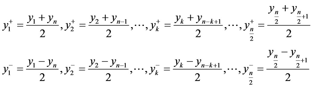
For the further discussion of these symmetries and related simplifications, it would be convenient at first to take into account the conservation laws, expressing the scattering amplitude as a function of independent variables only. After decomposition of the three-dimensional particle momentums in c.m.s. frame to components, which are parallel  and orthogonal
  to collision axis, and lets name them longitudinal and transversal momentums, respectively.
Energy of each particles in the finite state can be expressed by their momentum using the mass shell conditions, having  particles in finite state Figure 2, that give us
  momentum components of these particles. Since we are looking for a constrained extremum, it is necessary to take into account four relations, which express an energy-momentum conservation law. It will result in the fact that amplitude Equation (4) can be represented as a function of
  independent variables. The first 3n variables we choose are longitudinal and transverse components of momentums
 , of particles produced along the “comb“ in Figure 2. The other two variables are the transverse components of momentum
 .
.
If z-axis coincides with momentum direction  in c.m.s. and x and y axes are the coordinate axes in the plane of transverse momentums, the conservation laws look like
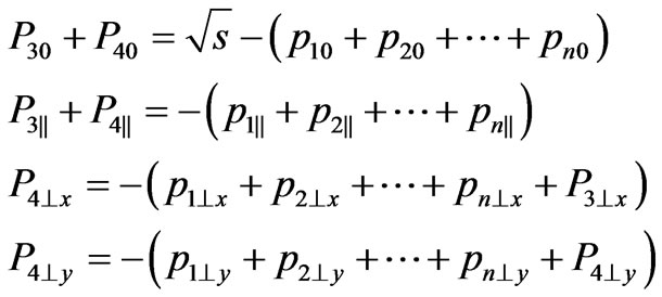 (5)
(5)
with
 (6)
(6)
Let’s enter the following denotations:
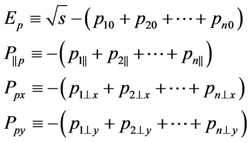 (7)
(7)
Then solving the system Equation (5) for the unknown ,
,  ,
,  ,
,  , we have:
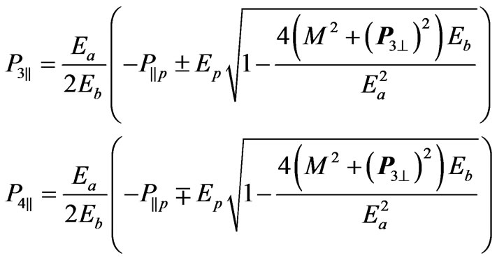 (8)
(8)
where
 (9a)
(9a)
 (9b)
(9b)
 (9c)
(9c)
We will discuss the choice of sign in Equation (8) further in the paper. Note that the value of  will not change, if we change the signs of all transversal momentums in Equation (8) simultaneously.
Substituting  from Equation (8) to Equation (6), and resulting
  from Equation (6) into Equation (4), give us the scattering amplitude as a function of independent variables, for which the conversation laws of all components of energy-momentum four-vector are taken into account. Below, referring to Equation (4), we assume that these substitutions have already been done. Taking into account this fact, we can define the amplitude Equation (4) as
 (10)
(10)
enumerating only independent variables in the argument list. When the scattering amplitude will be expressed in terms of independent variables only, it is possible to find the ordinary extremum, but not constrained extremum.
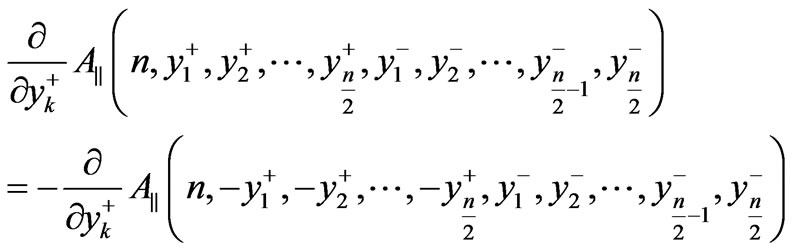
Now let us examine symmetries of the scattering amplitude in c.m.s. Obviously, the system has a symmetry under rotations around the collision axis, it means that there is no preferred direction in the plane orthogonal to collision axis. Hence, if the scattering amplitude has the constrained maximum point, it must be achieved at zero values of the particle momentums components in finite state transversal to collision axis. Otherwise these momentums must be somehow directed in the plane of transversal momentums, while all directions are equivalent in this plane.
To show more formally previous conclusion we use an explicit form of amplitude Equation (4), which transforms to itself, when the signs in front of all transversal momentums are changed:
 (11)
(11)
Take derivative from Equation (11) with respect to any of transversal momentum arguments and after that assuming all transversal momentums equal to zero, we obtain that all partial derivatives with respect to transverse momentum arguments are equal to zero if this arguments are equal to zero.
Thus, for the further search of the constrained maximum we can limit ourselves to reduction of the scattering amplitude on a subset of the values of its independent arguments, which corresponds to zero values of transversal momentums of all particles in finite state. This reduction is a function of longitudinal components of momentum  which we designate as
  and from Equation (4) we get:
 (12)
(12)
where
 (13a)
(13a)
 (13b)
(13b)
 (13c)
(13c)
 (13d)
(13d)
At the same time, assuming that all transversal momentums equal to zero, we have from Equation (8):
 (14)
(14)
Moreover, we have in c.m.s.  and
and
 , where s is determined in Equation (6).
For the further analysis it is convenient to switch from longitudinal momentums of secondary particles to rapidities , defined by following relation:
 . (15)
The function  can be written as
  . The initial state in c.m.s is symmetric with respect to changes in positive direction of collision axis. In addition, those type of diagrams of presented in Figure 2 have an axis of symmetry shown in Figure 3 for the case of even number Figure 3(a) and for the case of odd number Figure 3(b) of secondary particles.
From the explicit expression for amplitude Equation (12) can be shown that this expression will transform to itself, if we place instead the rapidity of every particle, the rapidity of particle symmetrically arrangement along the axis of symmetry Figure 3 and at the same time change the rapidity sign. Other words, if we change the variables for even number of particles
 (16)
(16)
the expression of restriction amplitude  will transform to itself. In case of odd number of particles the transformation similar to Equation (16), but instead of the rapidity
  which forms the axis of symmetry in Figure 3, must be substituted
  into the expression for the amplitude. The examined features of function
 can be expressed in the following symmetry relations for even number
  of secondary particles:
 (a) (b)
Figure 3. An elementary inelastic scattering diagram in the multi-peripheral model with even (a) and with odd (b) number of particles on the “comb” and it symmetry axis.
 (17)
(17)
and for odd number of secondary particles , respectively
 (18)
(18)
Proof of symmetry relations Equation (17) is given in Appendix B.
Now let us switch to new variables for even number of .
.
 (19)
(19)
and for odd number of 
 (20)
(20)
In these variables, the symmetry relation Equation (17) becomes
 (21)
(21)
and relation Equation (18) becomes
 (22)
(22)
Computing step by step the partial derivative of function Equation (21) with respect to variables ,
, , ···,
  , we obtain
 (23)
(23)
where .
.
It follows from relation Equation (23) for zero values of  the derivatives of the function

vanish. In the same way it can be shown that in case of odd number  of particles that for zero values of
  the derivatives of scattering amplitude

also vanishes.
This shows that for the extremum search we can consider a further reduction of the scattering amplitude on a subset of zero values of variables . By virtue of Equations (20)-(21) on this subset we have
 ,
,  at even
  and
and ,
,
 at odd n. Designating this reduction as
  we obtain at even
 :
:
 (24)
(24)
and at odd n
 (25)
(25)
If we now examine the formula Equation (12) on subset, where reduction  is considered, we will have
  by virtue of Equation (7). And therefore instead of Equation (14) we have the following expressions:
 (26)
(26)
or
 (27)
(27)
Let us take into account that if we decompose all scalar square terms in denominators of Equation (4) they will include the following difference
 and negative Equation (27), chosen as the
  in the end will give us greater value in the denominator than in the choice of Equation (26). Therefore it is naturally to suppose that the main contribution to cross-section Equation (1) gives the range of constrained maximum point determined by the scattering amplitude, where
  and
and  are given by Equation (26), but not by Equation (27). Hence, considering the expression Equations (24) and (25) for the reduction of the scattering amplitude at zero transverse momentum region, and performing further transformations, we assume that
  and related with it
  are expressed in terms of the longitudinal momenta of secondary particles by the relation Equation (26).
After we move on to the appropriate amplitude reduction  both in case of diagrams with even and odd number of particles we obtain function of particles rapidities located above the axis of symmetry in the diagram. The considered features of symmetry make it possible to simplify the energy parametrization of virtual particles, to which correspond the transversal lines located above axis of symmetry of diagrams in Figure 3.
Applying symmetry relation and conversation of energy, it follows that on subset, on which the considered amplitude reduction  is defined, the energy corresponding to the line connecting
  and
and  vertices of the diagram in Figure 2 is equal to zero in case of even number of particles at any values of independent variables (on which
  depends). Similarly, for an odd number of particles the energy transferred along the line, which joins
  and
and  vertices, is equal to
 . The corresponding proof is given in Appendix C.
Taking into account these results, reduction of  for the diagram in Figure 2 with even number of particles can be written in the form, which is convenient for the further numerical and analytical calculations:
 (28)
(28)
where
 (29a)
(29a)
 (29b)
(29b)
 (29c)
(29c)
The similar expression in case of odd number of particles in comb looks like:
 (30)
(30)
As it follows from Equations (28)-(30), it is convenient for the further calculations to make all quantities dimensionless by mass . In dimensionless form, these relations were used for numerical and analytical solution of the extremum for the reduction of the scattering amplitude
 .
.
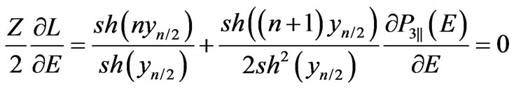
3. Numerical Solving the Constrained Maximum Problem for Multi-Peripheral Scattering Amplitude Squared Module
Numerical solution of the constrained extremum problem was done using Mathcad 2001 [12,13]. As it was shown in the previous section, since scattering amplitude corresponding to Figure 2 is real and positive, we can search for amplitude maximum instead the maximum of amplitude squared module. For cases of low values of secondary particles  we search not for the maximum of reduction
 , but for the maximum of total amplitude
  defined by Equation (4) with allowance for Equation (14) with the choice of positive sign in the front of
  (in order to transform this expression to Equation (26), when the symmetry properties will be taken into account). These calculations are numerical verification of validity of the discussed above simplifications related to the symmetry properties. A typical result of such calculation for the case of
  and energy
  GeV using Maximize function of Mathcad 2001 is shown in Table 1. As it follows from Table 1, the numerical

Table 1. A typical output of numerical computation of the maximum point of scattering amplitude corresponding to the diagram presented in Figure 2.
computation confirms above conclusion that all the transverse momentums must vanish at the maximum point. Note also that the set of rapidities corresponding to the maximum point in Table 1, which are determined by numerical computation, confirms conclusion that the diagrams centered at the axis of symmetry have mutually opposite values in the point of rapidity extremum. Similar results were obtained for different numbers of particles  and energies
 .
.
Now let us examine properties of the constrained maximum point following from the results of numerical computations. Some typical results are shown on Figure 5 and corresponding to it Table 2.
The column y in Figure 5 contains the rapidities of particles obtained using Maximize procedure (Mathcad) for which scattering amplitude  defined by Equation (28) in the case of even number particles and by Equation (30) in the case of odd number particles has maximum reduction. Moreover, note that the order of numbers in the columns match to the order of arguments in the corresponding function.
For instance, in Figure 4 at  the reduction determined by Equation (28) is the function of 15-teen variables
  corresponding to the particles rapidities joined to the upper 15-en vertices of the diagram in Figure 2. The column shown in Table 2 contains fifteen numbers, in which the function
 has a maximum and at the same time the first number in the column is the value of
 , the second number is the value of
  etc.
etc.
As it is apparent from Figure 4, there is an interesting

Figure 4. Rapidity dependence on vertex number in the diagram Figure 2 at the constrained maximum point.
 (a)
(a) (b)
(b)
Figure 5. The dependence of rapidity step Δy of an arithmetic progression, which constrainedly maximizing the scattering amplitude, on energy  for the different numbers n of particles on “the comb”. At high energies this dependence become logarithmic.


Table 2. Resulting rapidities obtained using Maximize procedure (Mathcad) for which scattering amplitude A0 defined by Equation (28) in the case of even number particles and by Equation (30) in the case of odd number particles has maximum reduction. The column Δy contains a difference between every column element and the successor of this column. The last column contains ratios yk/y15, k = 1, 2, ···, 15 and yk/y8, k = 1, 2, ···, 8.
feature, which consists in the fact that the maximizing rapidities in the case of even  and in the case of odd
 , are approximately equal to the numbers producing arithmetic progression. It is confirmed by the presented dependences in Figure 5.
  values are approximately equal to each other (see Table 2).
In addition, the proximity of the sequence of  column elements to an arithmetic progression follows also from calculations of
  and
and  columns, which are constructed by the following principle. If we assume that
  form an arithmetic progression with difference
 , in the case of even
  we obtain
 . On the other hand, from symmetry relations obtained in Section 2 we have
 . From these two relations we obtain
 . Then
  and in the similar manner
 , etc. Hence, in case of the diagram with even
  the rapidity ratios
  must form the sequence of odd whole numbers. The columns
  and
and  contains these ratios constructed by the column elements
  obtained with the help of Maximize function [12]. As seen from Table 2, the column elements
  and
and  are really close to odd numbers.
In case of odd  with allowance for
  we have
 (31)
(31)
Then the ratios 

 must produce the sequence of whole numbers 1, 2, ···. And Table 1, where columns
  and
and 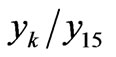 consist of such ratios, shows that these ratios are really close to the corresponding whole numbers. The similar results are obtained for different numbers of particles
  and energies
 .
.
The analytic form of arithmetic progression at any  and
and  will be considered in more detail below the text, when we will given an analytical solution of the extremum problem for reductions Equations (28) and (30).
Moreover, the results of numerical computations confirm the well-known multi-peripheral model assumption about particle rapidity ordering, because at the maximum point the particle rapidities monotone increase at movement upward along the diagram in Figure 2.
Besides of these results numerical computation allows to trace several other properties of the extremum point. In particular, if the rapidities in the maximum point form an arithmetic progression, the question arises, how the difference  of this arithmetic progression depends on the energy
  and the number of particles
 ? Result of numerical computation of the dependence of difference of an arithmetic progression
  on
on  at different numbers of particles on the “comb” Figure 2 are shown in Figure 5. At the same time the arithmetical average of column elements
  (the similar to shown in Table 2) was used as the value of
 .
.
As it’s obvious from Figure 5, the  is a monotonically increasing function of energy
  for a fixed number
  of particles. At the same time the dependence
  has some energy threshold.
It is obvious, that at given  such dependence makes sense only at
 (32)
(32)
(where  is not dimensionless by m), that corresponds to the total rest energy of particle in finite state. Note that function
 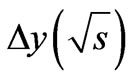 reaches asymptotic quite quickly. Since Figure 5 has a logarithmic scale on the energy axis, its seen that this asymptotic behavior is characterized by the linear dependence on logarithm of energy normalized to 1 GeV.
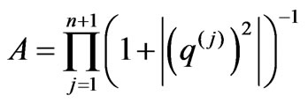
Output computation of the dependence of difference of an arithmetic progression  on the number of particles for set of energies
  = 10 GeV, 100 GeV, 1000 GeV is presented in Figure 6. From Figure 6 (where dependences
  are given in linear and logarithmic scales) it is evident that, when
  is small in comparison with the boundary value determined by Equation (32), this dependence is close to inversely. In particular, if we examine
  as a function of
 , it is possible to calculate corresponding difference of an arithmetic progressions for the given energy (they are marked as
  in Figure 8). As it follows from Table 3, ratios
 (33)
(33)
where  are close to (−1), which suggests that if we fix
  and examine
 , that is much smaller value than the maximum allowable by

Table 3. The difference of rapidity Δy from Figure 6. From these results it is evident that the dependence is close to inverse proportion.
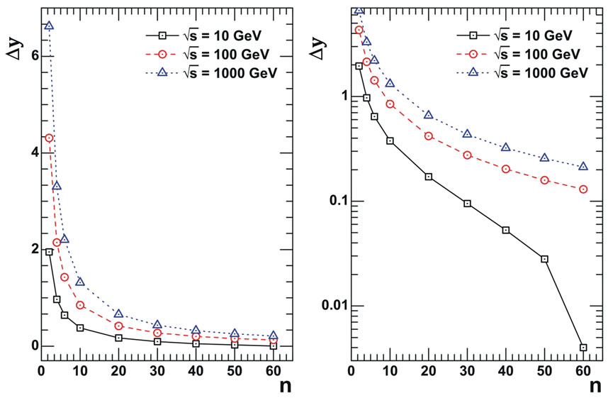
Figure 6. Dependence of difference Δy in an arithmetic proession, which constrainedly maximizing the inelastic scattering amplitude for the different number of particles n on the “comb” at the fixed energies : 10 GeV, 100 GeV and 1000 GeV.
law of conservation of energy for a given value , then we have
 .
.
More specific information about the dependence
 can be obtained from analytical solution of the constrained extremum problem for scattering amplitude, which will be considered in the next section.
However, the greatest interest is the dependence of the absolute values of virtualities on energy (i.e. the virtual particle squared four-momentums corresponding to the diagram in Figure 2, calculated at values of real particle four-momentums for which the scattering amplitude has a constrained maximum). Discussion of this problem leads us to possible mechanism of inelastic scattering cross-section growth with energy.
Let us designate the virtual particle four-momentums according to Figure 2:
 (34)
(34)
The numbers of four-momentums are taken in brackets to distinguish them from the four-momentum components notation. For example, notation  denotes zero component of contra variant four-vector
 .
.
As was noted above, all the quantities were made dimensionless by the mass  before calculations, therefore we introduce the notation
 (35)
(35)
At the same time the magnitude , which is determined by Equation (4) and coincident with scattering amplitude accurate within constant, can be written in dimensionless form like:
 (36)
(36)
From numerical computation we know particles fourmomentums in finite state, for which function  has constrained maximum. Therefore, with help of relations Equations (34) and (35) we can calculate four-momentums
  and whereupon calculate the corresponding dimensionless virtualities. Results of such calculation presented on Figures 7 and 9.
 (a)
(a) (b)
(b)
Figure 7. The virtuality variation along “the comb”. (a) shows particles virtuality dependence on vertex number on diagram Figure 2, for even number of particles (n = 20). Only the upper half of the diagram was considered, because as it follows from symmetry relations, discussed in Section 2, virtualities at the maximum point on the lines symmetrical to symmetry axis are equal. This also evident from (a), which shows the virtuality variation along the whole “the comb” for odd number of particles (n = 7).

Figure 9. Variation of the modulus of virtuality on energy for n = 20 at different energies.
As it well known, that there is reference frame where the particle energy vanishes [11] for particles with negative virtuality. Such a reference frame is called the standard reference system according to terminology of [11]. Obviously that the particle momentum in the standard reference system has the smallest possible value of all inertial frames of reference, and this smallest value is defined by particle’s virtuality.
Taking into account the Heisenberg uncertainty principle, we find that the virtuality characterizes a size of the domain, in which a particle can be detected with high accuracy, if the measurements were made in the standard reference system of this particle. At the same time, the more particle‘s virtuality, the smaller this size. Thus, the virtuality of particles makes it possible to judge the spatial extension of those domains, where inelastic processes take place described by the diagrams of type Figure 2. These space domains form the virtual “coats” of colliding particles, therefore these spatial extensions define typical sizes of colliding particles  and
and , see Figure 2. From Figure 7 it is evident that virtualities increase with movement from the diagram edges to its center. This is easy to explain, because all the virtualities are negative and therefore
 (37)
(37)
Taking into account that transversal components of momentum are equal to zero at the maximum point, we have:
 (38)
(38)
According to the law of conservation of energy we have . At the same time

and
 therefore
 . Since both these expressions are positive, we have
 . Therefore due to positivity of expressions in brackets, we obtain from Equation (38):
 . (39)
However, when we move from  to
to , we subtract
  from the lower side
  and
and  from the higher side
 . Consequently, the difference of these quantities increases, and so naturally to expect that the difference of squares, i.e., virtuality
 , increases too Figure 7. Turning to each subsequent virtuality, we will subtract a hyperbolic cosine of corresponding rapidity from the energy and subtract a hyperbolic sine of the same rapidity from the longitudenal momentum. The difference between the longitudinal momentum and the energy will increase, which explains the increase in the differences of their squares, i.e. virtualities.
Behavior of virtuality at the maximum point for different energies is shown in Figure 9. From the results in Figure 9, it follows that at the maximum point the virtuality monotone decreases with the energy growth. As it is evident from Equation (36), that the decrease of the virtuality should lead to amplitude increasing with energy at the maximum point, and for reasons outlined in Section 1 this should lead to increase of partial cross sections with energy  growth. Such an effect is a consequence of rapidity increasing at the maximum point, and therefore in principle cannot be taken into account within framework of multi-Regge kinematics [7,9,10,14] due to the fact that this dependence is neglected in the integrand of Equation (1).
Further, in the second part of our paper we will discuss the question of whether the amplitude growth can lead to growth in cross-section  calculated by Laplace method and in total scattering cross-section
 .
.
4. Analytical Solution of the Constrained Extremum Problem for Inelastic Scattering Amplitude at the Approximation of Equal-Denominators
We first consider in more detail the case of even number of particles n in the diagram of Figure 2. The scattering amplitude reduction  defined by Equation (28) undimensioned by mass
  takes a form:
 (40)
(40)
Here  and instead of
  and
and  we use their dimensionless by mass m values. Since we search for the constrained extremum, under condition of energy-momentum conservation, it is assumed that
  is described by Equation (26), in which again all values are undimensioned by mass
 . In particular, taking into account the symmetry relation, normalization and the introduction of rapidity (see Equation (15)), we obtain for
  instead Equation (7):
 (41)
(41)
For further calculations we use the following denotation
 and
and  (42)
(42)
Note that due to Equations (26), (41) and (42) quantity  depends on rapidity as the composite function of E, which is denoted as
  and the first term of Equation (40) depends on rapidity only via
 .
.
Instead of looking for the maximum of function  we can look for the maximum of its logarithm, which we define as
 :
:
 (43)
(43)
In addition, we make following denotation:
 (44)
(44)
Since after taking into account Equation (7), all variables of function  and hence logarithm became independent, then the extreme point can be found under condition that partial derivatives with respect to all variables are equal to zero. The equations for the extreme point problem can be written down in a form:
 (45)
(45)
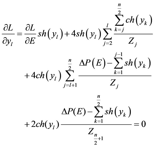 (46)
(46)
where .
.
 (47)
(47)
Equations (45)-(47) form the system of equations for the extreme point search. An approximate solution of this system is the purpose of this section. The simplification of this system of equations can be attained in approximation, which we call “the equal-denominators approximation”.
As seen from Equation (36), the amplitude is a product of fractions whose denominators contain the expression greater than unit. However, function  slowly varying at
 , that follows from its derivative. In addition, as discussed in Section 3, virtualities increase, and hence, as it evident from Equation (38) and arguments made after this relation, the denominators increase with movement from the edges of the “comb” to its center. However, as we are looking for the maximum point, virtualities at this point should be as small as possible. Therefore, they should increase as we move from the edges of the “comb” to the center as slowly as possible. Hence, we can expect that the denominators lightly differs from each other in the desired maximum point, then for the further analysis of the system of equations at the maximum point we adopt an approximation, in which all the denominators are equal between themselves. Their approximate common value will be denoted as
 ,
,
 . (48)
The equations for the maximum point as result of the approximation take form
 (49)
(49)
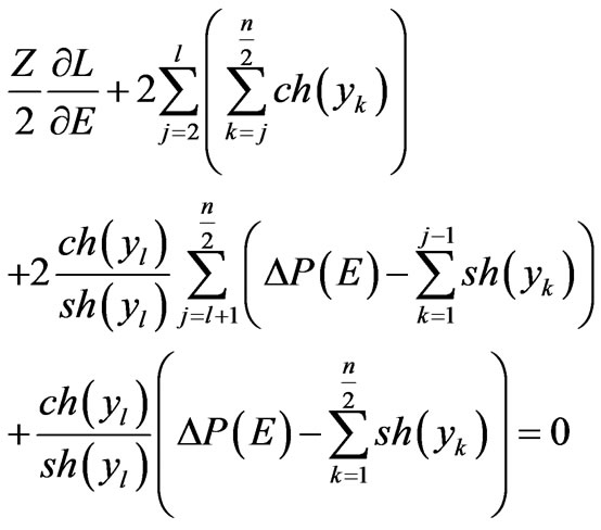 (50)
(50)
here 
 (51)
(51)
From approximation Equation (48), in particular, we obtain . Taking into account the notation Equation (44) leads to equality:
 (52)
(52)
Substituting Equation (52) to the system of equations Equations (49)-(51) we have
 (53)
(53)
 (54)
(54)
here 
 (55)
(55)
Equations (53)-(55) form a system of equations for search the point of the constrained maximum of inelastic scattering amplitude as approximation of equal denominators Equation (48). To solve this system we consider Equation (54), which corresponds to :
:
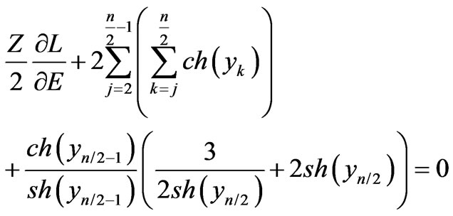 (56)
(56)
Subtracting Equation (56) from Equation (55) we get
 (57)
(57)
From this relation follows that
 (58)
(58)
Taking into account that a hyperbolic tangent is a monotonous function on whole real axis, from Equation (58):
 (59)
(59)
Note that this result agrees with the numerical results shown in Figure 4 and related to it Table 2 (see column  for n = 30). Now let us prove by induction that
 (60)
(60)
In the Equation (60) is already proved at k = 1, since it coincides with Equation (59). Let us assume that this equation is true for
 (i.e., at
 ) and prove that it is true at k = n/2 − l (i.e., at
 ).
).
Subtracting Equation (54) from Equation (55) we obtain:
 (61)
(61)
Note, that sums  and
and  under
under
 include only those
 , that covered by induction hypothesis. Then from Equation (60) we have
 . This makes it easy to calculate the sums from Equation (61), which after transformations takes a form:
 (62)
(62)
It follows that
 (63)
(63)
i.e., it coincides with proved Equation (60).
Thus, for diagrams with even number of particles we have shown that in the approximation of equal-denominators (see Equation (48)) analytically can be reproduce results shown in the previous section of numerical computation that rapidities at the maximum point form an arithmetic progression and that ratios of all rapidities to the minimum rapidity form the sequence of odd integers.
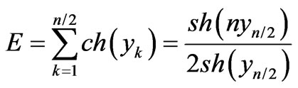
In order to determine the values of r pidities, for which scattering amplitude has a constrained maximum we still need to calculate the value , used to express all rapidities. This can be done using the equal-denominators approximation Equation (48).
Calculating the sums in Equation (55) with allowance for Equation (60), we have:
 (64)
(64)
Now using relation Equation (60) for the  we calculate the derivative
 . The corresponding expression will be looks like:
 (65)
(65)
 (66)
(66)
Using the equal-denominators approximation Equation (48), we obtain:
 (67)
(67)
 (68)
(68)
Taking into account Equation (52), after transformations we get:
 (69)
(69)
Put Equation (69) into Equation (64), we simplify obtained equation to form
 (70)
(70)
Derivative  can be calculated from Equation (26) with allowance for Equations (41) and (42). Based on these relations expression for
 , which is made dimensionless by mass
 , can be written as
 (71)
(71)
where it is assumed that the values  and particle masses
  at the ends of the “comb” are also made dimensionless by mass
 . Recall that in the numerical calculations described in previous section pion mass was set to
  and proton mass — to
 ).
).
Calculating the derivative of Equation (71) and put it into Equation (70), we obtain the equation, which after simple transformations reduces to the form:
 (72)
(72)
Note that the rapidity corresponding to momentum  is equal to
 , as it follows from Equations (71) and (72).
This expression would be obtained from Equation (60) if we accept , i.e., arithmetic progression Equation (60) lengthens by one term. We can say that the rapidities of particles in the ends of the “comb” at the maximum point “continue”, as it were, an arithmetic progresssion, formed by the rapidities of internal particles of the “comb”. This again indicates the close relation between the equal-denominators approximation Equation (48) and the fact that rapidities at the maximum point form an arithmetic progression. In other words, the arithmetic progression formed by rapidities at the maximum point is the result of equal-denominators approximation.
It is also possible to verify permissibility of this approximation in the following way. Taking into account that
 (73)
(73)
(as it follows from Equations (60) and (42) we get instead of Equation (72):
 (74)
(74)
This equation does not admit exact analytical solution, and further we will examine an approximate solution of this equation. However, we can verify permissibility of the approximations made above, which led to Equation (74), using Mathcad 2001 (or any other computer software for engineering and scientific calculations) to solve this equation numerically for different energies  and compare result with that was obtained in numerical determination of the maximum point and shown in Figure 5. The results of such comparison are shown in Figures 11 and 10.
As evident from Figures 10 and 11, the “exact” numerical solution of Equation (74) practically does not differ from the results of numerical computation. This means that equal-denominators approximation Equation (48), which leads to Equation (74) is admissible approximation.
Now let us consider an approximate analytical solution of Equation (74). Note that function
 in the left-hand side of Equation (74) varies slowly at small values of
  and can be
 (a)
(a) (b)
(b)
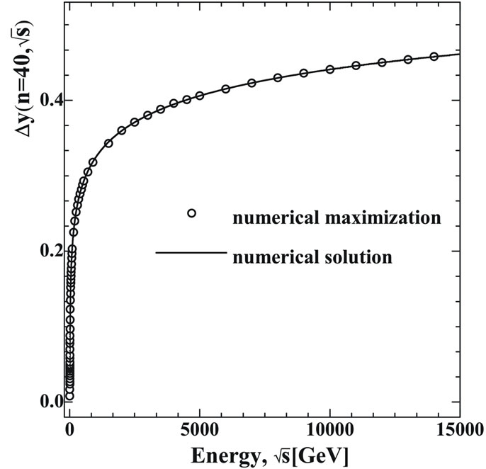
Figure 10. The numerical solution of Equation (74) (solid line) and numerical maximization (circles) of the magnitude  at n = 40 (10(a)) and n = 50 (10(b)).
replaced for the limiting value equal to  and
and  . In this approximation we obtain the following solution:
 (75)
(75)
The approximate solution of Equation (75) and the results of numerical computation are presented in Figure 11, where it is evident that Equation (75) gives a somewhat overstated value in comparison with numerical computation. It is naturally, because using approximation  in Equation (74), we underestimate value of function
  and thereby overstated the value of the hyperbolic cosine in the right-hand side of Equation (74).
Nevertheless, as evident from Figure 11, the absolute uncertainty of approximation Equation (75) does not increase with the energy growth, as the very of  increases, the relative error—falls. It can also be explained on the basis of Equation (74). Since
  becomes small in comparison with
  at sufficiently high energies
  (and
(and  accordingly) therefore, the accuracy of approximation of the function
  ceases to play a significant role. Neglecting
  in Equation (74) in comparison with
  and neglecting
  in Equation (75) in comparison with
  we obtain the same result. It means that approximation Equation (75) ensures the “correct” asymptotic of value
  at high
 .
.
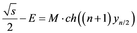
Let’s draw attention to some interesting features of Equation (75). Firstly, the approximate solution of Equation (75) has a threshold branch-point at  (dimensionless by mass
 ). This means that such a feature has a difference an arithmetic progression of the rapidity, for which inelastic process amplitude has maximum. The contribution of the considered inelastic processes to an imaginary part of the elastic scattering amplitude after calculation by Laplace method will be in some way expressed in terms of the difference of an arithmetic progression
 . Therefore we can expect that noted threshold feature will be included into the imaginary part of the elastic scattering amplitude via
 . And this feature is required by unitary condition.
Equation (75) has logarithmic asymptotic behavior at the high energies  and for the case when
  substantially exceeding a threshold value from Equation (75) we get
 , that coincides with the results of numerical computation (see Section 3).
For the diagram in Figure 2 with odd number of particles the sequence of iterations is similar to diagrams with even number of particles, which was described above.
At first we differentiate the logarithm of amplitude reduction Equation (30) with respect to all rapidities 

 . After that we can use the equal-denominators approximation
 (76)
(76)
From the condition of equality  we get relation similar to Equation (52):
 (77)
(77)
In view of Equation (77), in same way as we obtained Equation (58) from equality to zero of the derivatives of logarithm of scattering amplitude reduction with respect to  and
and  we get
 (78)
(78)
This result agrees with results of the numerical calculation presented in Table 2 (see column  for n = 17). Then, just as was done above, we can prove by induction that
 (79)
(79)
Thus all the rapidities, for which the considered scattering amplitude reduction has constrained maximum, can be expressed in terms of .
.
Making computation similar to those that led to the relations Equations (64)-(74) for this rapidity at the approximation of equal-denominators we obtain:
 (80)
(80)
In an approximation similar to that, which results in Equation (75), we get
 (81)
(81)
From Equation (81) it is evident that in the case of odd number n the rapidity difference of an arithmetic progression, for which scattering amplitude has constrained maximum, also has a threshold branch-point.
Note, that a difference of an arithmetic progression is equal to  in case of odd n and it is equal to
  in case of even
 , which shows in accepted approximation that difference of an arithmetic progression
  is expressed by the same relation as for the even
  and odd
 . The analytical results, which were obtained, allow us to trace how “works” the mechanism of virtuality reduction with the energy‘s growth. In approximation of equal-denominators Equation (48) with allowance for Equation (52) the amplitude value at the maximum point (in case of even
 ) can be written as:
 (82)
(82)
The quantity  included in this expression sets the characteristic value of virtuality at the maximum point of amplitude at the approximation of equaldenominators.
Taking into account increase of  with energy
  growth, which is approximately described by Equation (75), note that virtuality at the maximum point really decreases and the maximum value of amplitude grows with energy
  growth.
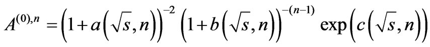
The demonstrated results were obtained in the approximation of equal denominator Equation (48). This approximation is acceptable in order to show that the scattering amplitude has a constrained maximum point and in order to find that maximum. However, to calculate the value of the amplitude at this point, this approximation provides insufficiently accurate result, so for the next section will be calculated amplitude at the maximum point in a more accurate approximation.
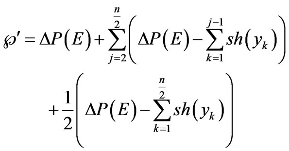
5. The Approximate Calculation of the Sum of Logarithms at the Point of Constrained Maximum
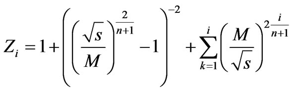
Taking into account the aforementioned results (see Figure 4 and Equations (60), (79)) for the calculation of constrained maximum point of multi-peripheral scattering amplitude, one gets the following representation of :
:
 (83)
(83)
where
 (84)
(84)
Through  we denote (as before) the difference of arithmetic progression at the point of constrained maximum. The aim of this chapter is to obtain the approximate solution for the
  which enters the exponent of Equation (83).
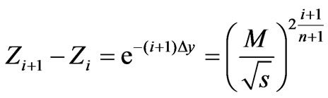
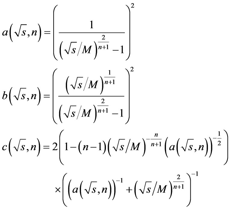
In the previous sections (see Figures 7 and 9) has been shown that Feynman denominators grow if one moves from comb’s edges to its center. In other words, the maximum of  values Equation (84) is
 . Furthermore, since Feynman denominators are obliged to grow while moving towards the comb’s center, the maximum of scattering amplitude is attained when the aforementioned growth is minimal. This means that the denominators at the point of maximum differ little from each other.
The results of numerical calculations enable to claim that the higher is the energy, the smaller is the difference of each Feynman denominator from the central one on the comb, with the exception of two outermost denominators (see Section 3 and Figures 7 and 9). This can be also shown analytically (see Equation (105)) Thus, one can try to express all denominators except two outermost ones in terms of .
.
 (85)
(85)
Taking into account that  differs little from
 , we get
 (86)
(86)
Substituting approximation Equation (86) into expression for scattering amplitude leads to:
 (87)
(87)
where
 (88)
(88)
 (89)
(89)
Equations (87)-(89) are expressing scattering amplitude in terms of solution  of transcendental Equation (74). Our next goal is to express scattering amplitude
  in terms of energy
 , the parameter which is characterizes the scattering process. Furthermore, we can restrict ourselves to considering energies far from threshold
 . This is due to the fact that near the threshold the behavior of partial cross-section is determined mostly by the volume of final-state particles phase space, which vanishes in the limit of
  , while
  remains restricted with some non-zero value. Therefore, the exact value of magnitude
  at such energies is insufficient.
6. The Approximate Solution of the Transcendental Equation Expressing the Difference of Rapidity Arithmetic Progression at the Point of Constrained Maximum of the Scattering Amplitude
Consider the transcendental equation Equation (74) taking into account the fact that . At energies sufficiently higher the threshold value, when is
  not small anymore, the energy of final-state protons
 (90)
(90)
is much higher than the pions energy
 .
.
which is caused with the greatness of proton mass  (in the units of pion mass) and with the fact that at not small
  one gets
 (91)
(91)
while
 (92)
(92)
The fact that most of energy in c.m.s. framework is carried by secondary protons in its turn means that the rapidity of each of these protons is close on absolute value to initial proton’s rapidity (let’s denote it ).
).
Namely,  (see Figure 12). Let’s enter the new variable instead of
 (93)
(93)
Taking into account  we’ll representEquation (74) as
 (94)
(94)
Neglecting the small magnitude  with respect to large magnitude
  one gets
 (95)
(95)
Taking into account the smallness of 
 (96)
(96)
Since the arguments of hyperbolic sine and cosine functions are large
 (97)
(97)
or
 (98)
(98)

Figure 12. The dependence of difference between initial and final-state protons rapidities on energy , calculated in the point of constrained maximum of scattering amplitude at n = 10 (solid line), and n = 20 (dash line).
In order to control the applicability of made above approximations let’s compare the solution of Equation (98) with the one, which can be obtained from Equation (93) substituting the “exact” solution of transcendental Equation (74) (where ). The result of such a comparison for n = 10 is depicted on Figure 13. These results enable to conclude that the entered approximations are applicable at least for rather high multiplicity of final-state particles.
Now we can pass to the approximations for other magnitudes, which enter to Equation (87), expressing the aforementioned scattering a multitude at the point of constrained maximum.
7. The Analytic Representation of Feynman Denominator at High Energies
Now, it is possible to analytically show the applicability of transformation Equation (86). The Feynman denominators on the comb may be represented as follows
 (99)
(99)
where
 (100)
(100)

Figure 13. The comparison of approximate solution of Equation (98) (circle) with results of numerical solution of Equation (74) with respect to magnitude ΔY (solid line) at n = 10.
If we consider the energies higher than threshold one
 we can neglect the product of two small quantities in this expression. Then we get
 (101)
(101)
Then, let’s consider the expression for . Taking into account Equation (93) one can represent Equation (88) as follows
 (102)
(102)
Taking into account Equation (97) we get
 (103)
(103)
Substituting Equation (103) into Equation (101) will result in
 (104)
(104)
or
 (105)
(105)
Namely, one can see that at high energies the difference between Feynman denominators falls exponentially. In other words, at high energies, the largest change of Feynman denominator occurs at the movement from zero (1st on the comb) to 1st (2nd on the comb) denominator. The result Equation (105) is illustrated on a Figure 14.
8. The Analytical Expression for Scattering Amplitude Dependence on Energy  at the Point of Constrained Maximum
In the previous analysis among the other results we derived an expression for  Equation (103). In order to verify a precision of this approximation we’ll compare it with an exact solution which can be obtained from Equation (88) by substituting the solution of transcendental Equation (94). As one can see from Figure 15 this is an adequate approximation.

Figure 14. The comparison for the magnitude of Feynman denominator jump on the comb at the point of constrained maximum obtained in the approximation Equation (105) (dashed lines with boxes and circles) with its exact value (red line) for n = 10 at  = 50 GeV and at
  = 200 GeV (blue line).

Figure 15. The dependence of (1/Z0)2 on energy  at n = 10 obtained from Equation (88) by substituting the solution of transcendental equation (Equation (74)) solid line; with the approximation Equation (103) boxes.
Thus, we got  described analytically. Now let’s get an analytical expression for two other multipliers entering to Equation (87). First we’ll rewrite
  Equation (89) in form
 (106)
(106)
Neglecting as before  with respect to
  and taking the common factor
  out of the brackets we get:
 (107)
(107)
Neglecting the small exponential summands which enters to hyperbolic sine and cosine leads us to:
 (108)
(108)
Again, the obtained approximation is compared with the results of numerical calculations Figure 16. Now the only thing left is to represent

in a more convenient form. First let’s rewrite it as follows:
 (109)
(109)
Performing the same trick as before, namely, neglecting  with respect to
  and getting rid of small exponential summands we get:
 (110)
(110)
Similarly
 (111)
(111)
Finally, lets gather all the results. Substituting Equations (103), (108), (110) and (111) into Equation (87) we get an analytic representation of scattering amplitude at the point of constrained maximum:
 (112)
(112)
where
 (113)
(113)
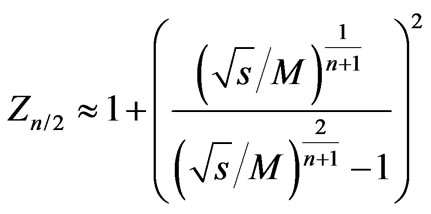
The  and
and  determine the characteristic value of virtuality at the maximum point of scattering amplitude and
  determines the variation of virtuality along the “comb“. In other words, the following estimate takes place
 (114)
(114)
where  is the absolute value of virtuality corresponding to j-th internal line on the “comb” in the point

Figure 16. The dependence of (Zn/2)−1 (a) an (Zn/2)− (n−1) (b) on energy  at n = 10. Solid line corresponds to Equation (89) with substituting the numerical solution of Equation (94), while dashed line refers to approximation Equation (108).
of constrained maximum. The comparison of scattering amplitude dependence on energy  obtained in analytical way with the one obtained by numerically solving Equations (83), (84) and substituting numerical solution of Equation (74) is presented on Figure 17.
Notation  was introduced to distinguish the exact value of amplitude defined by the relations relations Equation (83) and (84) from its approximate value Equation (112). To characterize the accuracy of approximation Equation (112) was introduced a relative deviation (see Figures 17(b) and (c)):
 (115)
(115)
9. Discussion and Conclusions
The main results and conclusion of this paper is that the multi-peripheral scattering amplitude indeed has a point of constrained maximum under conditions of the energy-momentum conservation law. This leads to the fact that the principal contribution to the multi-dimensional integrals, which representing the inelastic scattering cross-section with the production of a given number of particles, makes a small neighborhood of the maximum point.
Analyzing properties of the maximum point leads to some differences of the physical picture of the multiperipheral processes from ones, which leads to the basic formulas of Reggeon theory [5,8,15]. In particular, the rapidities of secondary particles at the maximum point are arranged and are equidistant from each other, as assumed in the justification of Reggeon formulas. At the same time in the presented model the distance between
the adjacent rapidities (i.e., difference of an arithmetic progression) depends on energy  and on number of particles
  (see Equations (75) and (81)), but not a constant value close to unity, as it accepted, for instance, in [5,8]. The assumption that the interval between adjacent rapidities does not depend on energy plays an important role for the ground of power dependence of the imaginary part of elastic scattering amplitude on Lorentz-invariant
 , that results in the Regge pole.
As it follows from Equation (114) energy term included in both sides is useful to rewrite it in this form
 (116)
(116)
It is obvious that the growth of exponent with energy  is much weaker than the corresponding decrease with the growth of number of particles
 . Thus, one can see that at not very small
  the value of
 even at high energies (
 ). As the result, the difference of energy and longitudinal momentum squares is at least not negligible with respect to transverse momentum for each virtuality on the “comb”. This result comes in contradiction with the statement that virtulalities can be reduced to transverse momentum squares, which is usually claimed in the standard approach [2-5,7-10].
Taking into account the growth of  with energy
  growth, we see that virtuality at the maximum point really decreases and the maximum value of amplitude grows with the growth of energy
 . Note also that at not very small
  the
the  is close to unity at rather wide energy range which results in the much steeper growth than the one which is attained in Regge-based theories [1,3,6,7, and 16] and described by factor of
 . Moreover, the higher
 , the wider is the energy range. Thus the asymptotic behavior for different
  is reached at different
  which enables to doubt the validity of the asymptotic formulas of multi-Regge kinematics.
In addition, as it follows from an examination of multi-peripheral diagrams in [3] and [5], Reggeon formulas are derived in case of total disregard to the dependence of the integrand for the cross section of production a certain number of particles on the rapidity of these particles. In such an approach a cross-section is defined by the value of rapidity phase volume. It is also well evident from the comparison of dependence of a set number particle production on  with the calculation of so-called volume of “transversal-truncated phase space” [2].
Obviously, that at the described above approach the dependence of scattering amplitude on rapidity is substantial, because just this dependence determines the value of scattering amplitude in the neighborhood of the most probable configuration of momentums.
Existence of the constrained maximum point in multiperipheral scattering amplitude and properties of this maximum allow us to apply this information for the calculation of inelastic scattering cross-section. This is the main purpose of our next paper.
Appendix A. The proof of Spatial Similarity of Virtual Particle Four-Momentums in the Diagram of Figure 2
We carry out the proof by “contradiction”. Suppose that any of the four-momentums of virtual particles, for example,  is time-like. Note that this four-momentum must be equal to
 by virtue of the law of energy-momentum conservation.
We assume that the time component of time-like four-momentum (energy) cannot vanish in any inertial system. This means that the sign of the time component of such four-momentum is the Lorentz-invariant quantity, i.e., cannot be changed when we move from one inertial system to another.
If we assume that the sign of the time components of four-momentum  (or four-vector
 ) is positive, the following inequalities must be simultaneously satisfied in all the inertial systems:
 (A1.1a)
 (A1.1b)
Given that both inequalities include the energy components of the energy-momentum four-vectors of real particles, satisfying to the mass shell conditions, we can rewrite them as
 (A1.2a)
 (A1.2b)
Note that first of these inequalities cannot take place in the rest frame of particle  because
 (A1.3)
If we assume that the time component of considered four-vector has a negative sign, then we obtain that in all inertial systems the following inequalities must be simultaneously satisfied:
 (A1.4a)
 (A1.4b)
However, second of these inequalities cannot take place in the rest frame of particle .
.
Thus, we can satisfy of energy-momentum conservation law in all inertial systems only in case, if the time component of considered four-vector changes a sign when moving from one reference frame to other. However in this case this four-vector cannot be time-like. Because presented argumentation is applicable to any of virtual four-momentums in the diagram Figure 2, they must all be space-like. Quod erat demonstrandum.
Appendix B. The Proof of Equation (17) from Section 2
Using function  defined by Equation (12), let us examine function
 , which is determined by relation:

(A2.1)
The expression
 (A2.2)
We would obtain if we were choose the direction of longitudinal momentum  as the positive direction of collision axis and interchange the four-momentums of particles in the diagram, arranged symmetrically about the axis in Figure 3 (numeration of the diagram vertices corresponds to Figure 2).
In order to write function Equation (A2.2) in explicit form, we will at first rewrite it in following way:
 (A2.3)
where
 (A2.4a)
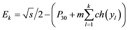 (A2.4b)
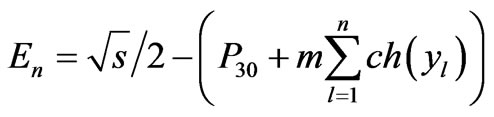 (A2.4c)
Moreover, as
 (A2.5)
with
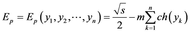 (A2.6a)
 (A2.6b)
then we obtain

(A2.7)
and accordingly

(A2.8)
With this we get
 (A2.9)
where
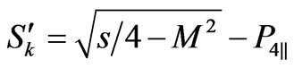 (A2.10a)
 (A2.10b)
 (A2.10c)
Or in more convenient form expression Equation (A2.9) looks like:
 (A2.11)
where
 (A2.12a)
 (A2.12b)
We take into account that amplitude depends on the rapidity, which satisfy the conservation laws of energy and longitudinal momentum components:
 (2.13)
From the conservation of the longitudinal component of momentum, we obtain
 (A2.14)
From the energy conservation low we have
 (A2.15)
and
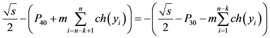 (A2.16)
Substituting Equations (A2.16) to (A2.11) we obtain:
 (A2.17)
where
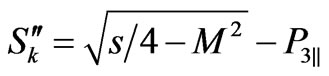 (A2.18a)
 (A2.18b)
 (A2.18c)
Replacing index k = n − j in product included in the expression for amplitude, we obtain the expression coincident with Equation (12) (taking into account Equation (15))
 (A2.19)
Taking into account Equation (A2.1), we obtain the required relation Equation (17):
 (A2.20)
Appendix C. Calculation of the Energies of the Virtual Lines That Intersect with the Axis of Symmetry of the Diagrams in Figure 3
Let us examine at first the case of an even number of particles. The law of conservation of energy in c.m.s has a form:

(A3.1)
Since constrained maximum of the scattering amplitude gives a symmetric configuration of ,
, 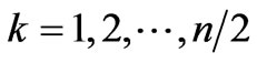 and
and 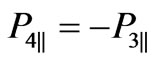 (that follows from Equaion (26)), then at the maximum point we get:
 (A3.2)
hence
 (A3.3)
However expression Equation (A3.3) corresponds to the energy transferred through the central link of the diagram between vertices with numbers of  and
and  (Figures 2 and 3); therefore this energy is equal to zero at the maximum point.
Now let ladder has odd number of particles . Writing the law of conservation energy, we select in the sum of pion energies the term corresponding to the central particle in the diagram:

(A3.4)
The maximum of inelastic scattering amplitude is reached at the symmetric configuration. It is characterized by the fact that the central particle has zero rapidity and the particles located symmetrically about the center particle have mutually oppositely rapidities, therefore
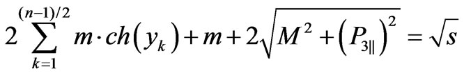 (A3.5)
It follows that
 (A3.6)
Thus, the energy, which flows between  -th and
  -th particles at the most probable configuration, is equal to
 . As
. As 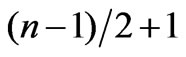 -th particle takes away energy
  (which has zero rapidity at the maximum point), then the following link in the diagram will be transferred energy
 .
.