Stability Analysis and Stochastic SI Modelling of Endemic Diseases

Desalegn Petros Kelkile

Pan Africa University Institute of Basic Sciences, Technology and Innovation, Nairobi, Kenya.

DOI: 10.4236/apm.2018.85030                

Abstract

In this paper, we study a stochastic epidemic model in Meta-population setting. The stochastic model is obtained from the deterministic model by set up random perturbations about the endemic equilibrium state. The outcome of random perturbations on the stability actions of endemic equilibrium is discussed. Stability of the two equilibriums is studied using the Lyapunov function.

Keywords

Meta-Population, Basic Reproduction Ratio, Lyapunov Function, Positive Equilibrium

1. Introduction

Modeling of infectious diseases with stochastic differential equation (SDE) has increased foundation lately due to its extensive variety of applications and its aptitude to reflect actuality in epidemiology [1] . The diseases outbreaks in a population of susceptibles rationally go behind stochastic processes [2] . Stochastic process occurs naturally in lots of physical applications where randomness is to be incorporated in the mathematical model [3] [4] . In recent years, main studies on stochastic model that have been published by researchers have recognized the growing significance of study the stability of stochastic positive equilibrium, as well as the global stability of the endemic equilibrium [5] [6] [7] . In this paper we approached by using deterministic and stochastic model. Briefly deterministic models are model processes which are often described by differential equations, with a unique input leading to a unique output for well-defined linear models and with multiple outputs possible for non-linear models. Throughout this paper, let $\left(\Omega \mathrm{,}\mathcal{F}\mathrm{,}\mathcal{P}\right)$ be a complete probability space with a filtration ${\left({\mathcal{F}}_t\right)}_{t\in ℝ}$ satisfying the usual conditions (i.e., it is right continuous and increasing while ${\mathcal{F}}_0$ contains all $\mathcal{P}$ -null sets).

Considering the general n dimensional stochastic differential equation

$\text{d}x\left(t\right)=f\left(x\left(t\right),t\right)\text{d}t+\phi \left(x\left(t\right),t\right)\text{d}Bt$

on $t\ge 0$ with initial value $x\left(0\right)=x_0$ , the solution is denoted by $x\left(t\mathrm{,}{x}_0\right)$ . Assume that $f\left(0,t\right)=0$ and $\phi \left(0,t\right)=0$ for all $t\ge 0$ , so (1.0) has the solution $x\left(t\right)=0$ . This solution is called the trivial solution.

Definition 1.1. The trivial solution $x\left(t\right)=0$ of (1.0) is said to be as follows:

1) stable in probability if for all $ϵ>0$ ,

$\underset{x_0\to 0}{lim}\mathcal{P}\left(\underset{t\ge 0}{sup}\left|x\left(t\mathrm{,}{x}_0\right)\ge ϵ\right|\right)=0$

2) asymptotically stable if it is stable in probability and, moreover,

$\underset{x_0\to 0}{lim}\mathcal{P}\left(\underset{t\to \infty }{lim}x\left(t\mathrm{,}{x}_0\right)=0\right)=1$

3) asymptotically stable in the large if it is stable in probability and, moreover, for all $x_0\in ℝ$

$\mathcal{P}\left(\underset{t\to \infty }{lim}x\left(t\mathrm{,}{x}_0\right)=0\right)=1$

In this paper, we consider the epidemic model in Meta-population setting. From the proposed schematics of the compartment model shown in [8] , we will extract a metapopulation model for HIV dynamics among the youth coupled with awareness/education i.e., we extended the single patch disease model to include multiple patches (see Figure 1).

Figure 1. A schematic of the metapopulation model. A schematic of the metapopulation model for HIV transmission in the youths coupled with awareness/education in each patch i, i = 1, ・・・, n.

Differential Equation of the Model

States variables: $S_C$ , susceptible children, $S_{YUF}$ , susceptible uneducated female youth, $S_{YUF}$ , susceptible educated female youth, $S_{YUM}$ , susceptible uneducated male youth, $S_{YEM}$ , susceptible educated male youth, $I_C$ , infected children(children who were infected either during pregnancy or at childbirth), $I_{YUF}$ , infected uneducated female youth, $I_{YEF}$ , infected educated female youth, $I_{YUM}$ , infected uneducated male youth, $I_{YEM}$ , infected educated male youth, and $T_Y$ , antiretroviral therapy treatment among the youths. Parameters: $\mu$ , death rate of the youth and children, $\delta$ , disease induced rate in the youth and children before ART, ${\delta }_1$ , disease induced deaths in the youth and children after ART, $\lambda$ , birth rate, $\theta$ , rate of vertical transmission, ${\beta }_1$ , probability a susceptible female youth gets infected by infected male youth, ${\beta }_2$ , probability a susceptible male youth gets infected by infected female youth, ${\phi }_1$ , rate at which children grow to become uneducated female youth, ${\phi }_2$ , rate at which children grow to become educated female youths, ${\phi }_3$ , rate at which children grow to become uneducated male youths, ${\phi }_4$ , rate at which children grow to become educated male youth, $\rho$ , awareness/education rate, $\alpha$ , rate at which infected youth take the ART. The solid lines represent movement between classes and the dashed lines represent rate at which a susceptible individual moves in to infected class.

The model answers one important underlying research subjects; the determination of the existence of the threshold parameter which hints on the spreading or dying out of an invading epidemic into a population of susceptible. In this research article, we first study the positivity and boundedness of the system (1.0). The basic reproduction ratio is determined. Applying the hypothetical theorem of the Lyapunov functional, we find out the global stability of the two equilibria for system (1.0). We extend our stability analysis to the stochastic system (5.0), which is obtained by random perturbation of the deterministic system (1.0) and find the stability of its positive equilibrium. Finally, numerical examples which shows the dynamics of systems (1.0) and (5.0) are given, which gives the explicit difference in the dynamics of the models.

2. Basic Properties of the Model

In this section, the basic properties of model system (1.1) which are useful in the proofs of stability are studied. These are the invariant region and positivity of solutions. The former describes the region in which the solutions of system (1.1) makes biological sense while the latter describes non-negativity of solutions of system (1.1). The model under consideration monitors a human population and as such, we need to have that all the parameters and the variables of the model are positive for all $t\mathrm{<mi>\; </mi>}\ge \mathrm{<mi>\; </mi>\; 0}$ .

2.1. Positivity of Solutions

The theory of ordinary differential equations requires that, for every set of initial conditions

$\left(S_{YUF\mathrm{,}{i}_0}\mathrm{,}{S}_{YEF\mathrm{,}{i}_0}\mathrm{,}{S}_{YUM\mathrm{,}{i}_0}\mathrm{,}{S}_{YEM\mathrm{,}{i}_0}\mathrm{,}{I}_{YUM\mathrm{,}{i}_0}\mathrm{,}{I}_{YEM\mathrm{,}{i}_0}\mathrm{,}{I}_{YEF\mathrm{,}{i}_0}\mathrm{,}{I}_{YUF\mathrm{,}{i}_0}\mathrm{,}{T}_{i_0}\right)$ the state variables $\left(S_{YUF\mathrm{,}i}\left(t\right)\mathrm{,}{S}_{YEF\mathrm{,}i}\left(t\right)\mathrm{,}{S}_{YUM\mathrm{,}i}\left(t\right)\mathrm{,}{S}_{YEM\mathrm{,}i}\left(t\right)\mathrm{,}{I}_{YUM\mathrm{,}i}\left(t\right)\mathrm{,}{I}_{YEM\mathrm{,}i}\left(t\right)\mathrm{,}{I}_{YEF\mathrm{,}i}\left(t\right)\mathrm{,}{I}_{YUF\mathrm{,}i}\left(t\right)\mathrm{,}{T}_i\left(t\right)\right)$ of the solution must remain non-negative.

Proposition 2.1 Let the initial data be

$\begin{array}{l}\{(S_{c\mathrm{,}i}>\mathrm{0,\; <mi>\; </mi>}{S}_{YUF\mathrm{,}i}>\mathrm{0,}{S}_{YEF\mathrm{,}i}>\mathrm{0,\; <mi>\; </mi>}{S}_{YUM\mathrm{,}i}>\mathrm{0,\; <mi>\; </mi>}{S}_{YEM\mathrm{,}i}>\mathrm{0,\; <mi>\; </mi>}{I}_{YUM\mathrm{,}i}>\mathrm{0,}\\ \mathrm{<mi>\; </mi>}{I}_{YEM\mathrm{,}i}>\mathrm{0,}{I}_{YEF\mathrm{,}i}>\mathrm{0,}{I}_{YUF\mathrm{,}i}>\mathrm{0,\; <mi>\; </mi>}{T}_i)\ge \mathrm{<mi>\; </mi>\; 0}\}\in \Omega \mathrm{.}\end{array}$

Then, the solution set

$\left\{\left(S_{YUF\mathrm{,}i}\left(t\right)\mathrm{,}{S}_{YEF\mathrm{,}i}\left(t\right)\mathrm{,}{S}_{YUM\mathrm{,}i}\left(t\right)\mathrm{,}{S}_{YEM\mathrm{,}i}\left(t\right)\mathrm{,}{I}_{YUM\mathrm{,}i}\left(t\right)\mathrm{,}{I}_{YEM\mathrm{,}i}\left(t\right)\mathrm{,}{I}_{YEF\mathrm{,}i}\left(t\right)\mathrm{,}{I}_{YUF\mathrm{,}i}\left(t\right)\mathrm{,}{T}_i\left(t\right)\right)\right\}$ of system (1.1) is positive for all $t\mathrm{<mi>\; </mi>}\ge \mathrm{<mi>\; </mi>\; 0}$

Proof. Let $\alpha ={\beta }_{\mathrm{1,}i}^U\frac{I_{YUM\mathrm{,}i}}{N_{YUM\mathrm{,}i}}$ $\gamma ={\beta }_{\mathrm{1,}i}^E\frac{I_{YEM\mathrm{,}i}}{N_{YEM\mathrm{,}i}}$ From the first equation of model

system (1.1),

$\frac{\text{d}{S}_{YUF,i}}{\text{d}t}=\mathrm{<mi>\; </mi>}\left(1-\Pi \right)\lambda -\alpha S_{YUF,i}-\gamma S_{YUF,i}-\left({\rho }_i+{\mu }_i\right)S_{YUF,i}$

That is,

$\frac{\text{d}{S}_{YUF\mathrm{,}i}}{\text{d}t}\ge \mathrm{<mi>\; </mi>}-\Pi \lambda -\left(\alpha +\gamma +{\rho }_i+{\mu }_i\right)S_{YUF\mathrm{,}i}$

Integrating (2.0) by separation of variables gives

${\displaystyle \int }\frac{\text{d}S}{S}\ge -{\displaystyle \int }\left(\Pi \lambda +\left(\alpha +\gamma +{\rho }_i+{\mu }_i\right)S_{YUF\mathrm{,}i}\right)\text{d}t$

$S\left(t\right)\mathrm{<mi>\; </mi>}\ge \mathrm{<mi>\; </mi>}S\left(0\right){\text{e}}^{-{\displaystyle \int }\left(\Pi \lambda +\left(\alpha +\gamma +{\rho }_i+{\mu }_i\right)S_{YUF\mathrm{,}i}\right)\text{d}t}>0$

This proves that $S\left(t\right)>0$ for all $t\ge 0$ . Similarly, it can be shown that the remaining variables of system (1.1) are also positive $\forall t>0$ .

Remark 2.1. ${\text{e}}^k>0$ for all $k\in R$ .

2.2. Invariant Region

Note that

$\frac{\text{d}{N}_i}{\text{d}t}\le 4{\lambda }_i-{\mu }_i{N}_i-{\delta }_{\mathrm{1,}i}{T}_i\le 4{\lambda }_i-{\mu }_i{N}_i$

We now apply Birkhoff and Rotas theorem on differential inequality (2.1). By separation of variables of differential inequality (2.1), we get

$\frac{\text{d}{N}_i}{4{\lambda }_i-{\mu }_i{N}_i}\mathrm{<mi>\; </mi>}\le \mathrm{<mi>\; </mi>}\text{d}t$

Integrating (2.2) on both sides gives,

${\displaystyle \int }\frac{\text{d}{N}_i}{4{\lambda }_i-{\mu }_i{N}_i}\mathrm{<mi>\; </mi>}\le \mathrm{<mi>\; </mi>}{\displaystyle \int }\text{d}t=\frac{-1}{\mu }\ln \left(4{\lambda }_i-{\mu }_i{N}_i\right)+c$

$ln\left(4{\lambda }_i-{\mu }_i{N}_i\right)\ge -\mu \left(t+c\right)$

Therefore,

$4{\lambda }_i-{\mu }_i{N}_i\mathrm{<mi>\; </mi>}\ge A{\text{e}}^{-\mu t}$

where A is a constant. Now, applying the initial condition $N\left(0\right)=N_{0i}$ in (2.3), we get

$A=4{\lambda }_i-{\mu }_i{N}_{0i}$

Substituting (2.4) into (2.3) gives

$4{\lambda }_i-{\mu }_i{N}_i\ge 4{\lambda }_i-\mu N_{0i}{\text{e}}^{-\mu t}$

Making N the subject in (2.5) we have,

$N\le \frac{4{\lambda }_i}{\mu }-\left(\frac{4{\lambda }_i-{\mu }_i{N}_{0i}}{\mu }\right){\text{e}}^{-\mu t}$

As $t\to \infty$ in (2.6) above, the population size N, approaches

$0\le N\le \frac{4{\lambda }_i}{\mu }\Rightarrow N\to \frac{4{\lambda }_i}{\mu }$

Therefore, the feasible solutions set of system (2.7) enters the region

$\Omega =\left\{\left(S_{YUF\mathrm{,}i}\mathrm{,\; <mi>\; </mi>}{S}_{YEF\mathrm{,}i}\mathrm{,\; <mi>\; </mi>}{S}_{YUM\mathrm{,}i}\mathrm{,\; <mi>\; </mi>}{S}_{YEM\mathrm{,}i}\mathrm{,\; <mi>\; </mi>}{I}_{YUM\mathrm{,}i}\mathrm{,\; <mi>\; </mi>}{I}_{YEM\mathrm{,}i}\mathrm{,\; <mi>\; </mi>}{I}_{YEF\mathrm{,}i}\mathrm{,\; <mi>\; </mi>}{I}_{YUF\mathrm{,}i}\mathrm{,\; <mi>\; </mi>}{T}_i\right)\mathrm{<mi>\; </mi>}\in \mathrm{<mi>\; </mi>}{R}_{+}^9\mathrm{<mo>\; :\; </mo>}{N}_i\mathrm{<mi>\; </mi>}\le \mathrm{<mi>\; </mi>}\frac{4{\lambda }_i}{{\mu }_i}\right\}$

In this case, whenever $N>\frac{4{\lambda }_{0i}}{\mu }$ , then $\frac{\text{d}N}{\text{d}t}<0$ which means that $N\mathrm{<mi>\; </mi>}\to \frac{4{\lambda }_{0i}}{\mu }$ . On the other hand, whenever $N_i\mathrm{<mi>\; </mi>}\le \mathrm{<mi>\; </mi>}\frac{4{\lambda }_{0i}}{{\mu }_i}$ , every solution with initial

condition in $R_{+}^9$ remains in that region for $t>0$ . Thus, the region is positively-invariant.

3. Basic Reproduction Number

The basic reproduction ratio ( $R_0$ ) is defined as an infections originating from an infected individual that invades a population originally of susceptible individuals.

The above system can be represented in matrix form as $I^{.}=fI+vI$ where f is the matrix of the infection rates and v is the matrix of the transition rates.

The spectral radius of the Metzler Matrix, $\rho \left(-F{V}^{-1}\right)$ , is defined as the largest eigenvalue of the Metzler Matrix. Thus:

$\rho \left(-F{V}^{-1}\right)=\left|\left(-F{V}^{-1}\right)-\lambda I\right|$

$R_1=\frac{{\beta }_{\mathrm{2,}i}^U\left(N_{YEM\mathrm{,}i}+N_{YUM\mathrm{,}i}\right)}{\left({\rho }_i+{\mu }_i+{\delta }_i\right)N_{YUF\mathrm{,}i}}$

If for j = 1, 2, 3, 4, then each infectious individual in Sub-Population j infects on average less than one other person and the disease is likely to die out Otherwise, If for j = 1, 2, 3, 4, then each infectious individual in Sub-Population j infects on average more than one other person; the infection could therefore establish itself in the population and become endemic. An SIR epidemic model, where the presence or absence of an epidemic wave is characterized by the value of.

4. The Global Stability of the Endemic Equilibrium

In this part, we analyse the global stability of the endemic equilibrium point by construction a appropriate Lyapunov function. For simplicity, we consider the reduced model system (6) to prove for global stability. We use the come up to of [8] as it is used for several complicated epidemiological models. We consider the Lyapunov function of the form

where (for i = 1, 2, ・・・, 6 is a properly chosen positive constant in the given region. is a population of compartment i and is the equilibrium level. So we define the Lyapunov function as

The time derivative of L is

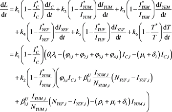
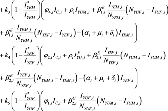
At an endemic equilibrium point we have

Therefore,

Simplification yields

let, where

F is non-positive by following the approach of [9] . Thus, for

. Hence and is zero when,

, , , ,. Therefore, the largest

invariant set in such that is the singleton which is our

endemic equilibrium point. By LaSalles invariant principle [9] we conclude that is globally asymptotically stable (g.a.s). Thus, we establish the following theory.

Theorem 3.1 When, the endemic equilibrium point is globally asymptotically stable in.

5. The Stochastic Model

Stochastic perturbations were bring in some of the major parameters involved in the model equations.

Here, we bring in stochastic perturbations in the major parameters of the deterministic model (1.1). Thus we permit stochastic perturbations of the variable

around their values at positive equilibrium. Hence, we assume that the white noise of the stochastic perturbations of the variable around values of are proportional to the distances of

from

Hence the stochastic version of model (1.1) is

With where are real constants, and

are independent wiener processes. We examine the asymptotic stability behavior of the equilibrium of the stochastic equation (5.0) and contrast results with the deterministic model (1.1).

Stochastic Stability of the Positive Equilibrium

It can be shown clearly that, the deterministic model (1.1) has one disease-free equilibrium

which is globally asymptotically stable when. However, when, the disease-free equilibrium is unstable. Obviously, there is also a unique positive endemic equilibrium

This equilibrium is globally asymptotically stable. The stochastic system (5.0) has the similar equilibria as the deterministic system (1.1). Assuming that, we examine the stability of the endemic equilibrium of (5.0). The stochastic differential equation (5.0) can be centered at its positive equilibrium by the change of variables

The linearized system of the stochastic model (5.0) around takes the form

where

and equals

Clearly, the endemic equilibrium corresponds to the trivial solution in (5.2). We denote L to be the differential operator associated with (5.2), defined for the family of nonnegative functions such that it is continuously differentiable with respect to t and twice with respect to x.

According to Afanas ev et al. [9] , the differential operator L for a function is given by

where

and

where, “T” and “Tr” are the transposition and trace respectively. With reference to Afanas?? ev et al. [9] , the following results hold.

Theorem 5.1: Suppose a function exist, satisfying the following inequalities

where and. Then the trivial solution of (5.2) is p^th moment exponentially stable. Again, given that p = 2 the trivial solution is supposed to be exponentially stable in mean square and the equilibrium x = 0 is globally asymptotically stable. From theorem 5.1, the conditions for stochastic asymptotic stability of trivial solution of (5.0) are given theorem 5.2.

Theorem 5.2: Suppose

and hold, then the zero solution of (5.0) is asymptotically mean square stable.

Proof: We consider the Lyapunov

where non-negative constants that will be chosen in the course of the proof. It can be easily ascertained that inequality (5.4) hold true when Applying the operator L on gives

Further

Now remark that

and

with

Now, from Equation (5.5), if we choose

and then from Equation (5.5), it is easy to verify that,

From the assumptions of the theorem, we deduce that and. Hence, D is a symmetric positive definite matrix. Let denote the minimum of its eleven positive eigenvalues, , , , , , , , , and; then,we can easily get

According to Theorem 5.1, we conclude that the trivial solution of stochastic system is globally asymptotically stable.

Hence, according to theorem 5.1, the proof is completed.

6. Conclusion

In this article, the dynamics of deterministic epidemic model and its stochastic variant are presented. The stability analyses of the deterministic model were investigated. Suitable Lyapunov functions were constructed for the global stability of the two equilibria. Mathematical analysis was done and it was established that in the absence of the disease a disease free equilibrium will always exist if for j = 1, 2, 3, 4,. We also established that the endemic equilibrium exists in the presence of the disease that is when for j = 1, 2, 3, 4, with the infectious population greater than zero. Reducing the infection in the vector population reduces for j = 1, 2, 3, 4, greatly. Thus the best methods of controlling HIV transmission is to target the Infected uneducated female youth, Infected educated female youth, Infected uneducated male youth, Infected educated male youth. is a threshold that completely determines the global dynamics of disease transmission. Our major purpose of the study was to examine the asymptotic stability behavior of the endemic equilibrium of the stochastic version of the deterministic epidemic model in Metapopulation setting.

Conflict of Interest

The author(s) declare(s) that there is no conflict of interest regarding the publication of this paper.

Conflicts of Interest

The authors declare no conflicts of interest.

References

[1]	Damian, C. (2005) A Stochastic SIS Infection Model Incorporating Indirect Transmission. Journal of Applied Probalility, 42, 726-737. https://doi.org/10.1239/jap/1127322023
[2]	Carletti, M. (2007) Mean-Square Stability of a Stochastic Model for Bacteriophage Infection with Time Delays. Mathematical Biosciences, 210, 395-414. https://doi.org/10.1016/j.mbs.2007.05.009
[3]	Liu, X.Q., Zhong, S.M., Tian, B.D. and Zheng, F.X. (2013) Asymptotic Properties of a Stochastic Predator-Prey Model with Crowley-Martin Functional Response. Journal of Applied Mathematics and Computing, 43, 479-490. https://doi.org/10.1007/s12190-013-0674-0
[4]	Gregory, F.L. (1995) Introduction to Stochastic Model. Chapman and Hall, London.
[5]	Lahrouz, A., Omari, L. and Kiouach, D. (2011) Global Analysis of a Deterministic and Stochastic Nonlinear SIRS Epidemic Model. Nonlinear Analysis: Modelling and Control, 16, 59-76.
[6]	Das, P., Mukherjee, D. and Hsieh, Y.H. (2011) An S-I Epidemic Model with Saturation Incidence: Discrete and Stochastic Version. International Journal of Nonlinear Analysis and Applications, 1-9.
[7]	Mukherjee, D. (2003) Stability Analysis of a Stochastic Process for Prey-Predator System with Disease in the Prey. Nonlinear Analysis: Modelling and Control, 8, 83-92.
[8]	Desalegn, P. (2018) Stability Analysis of a Deterministic Epidemic Model in Metapopulation Setting. Advances in Pure Mathematics, 8, 219-231. https://doi.org/10.4236/apm.2018.83011
[9]	Afanasev, V.K., Kolmanowski, V.R. and Nosov, V.R. (1996) Mathematical Model of Global Systems Design. Kluwer, Dordrecht.