1. Introduction
In recent years, physical acoustic wave modeling has become a successful tool in diagnostic and therapeutic ultrasound application. There are several wave equations available for describing acoustic wave propagation [1-4]. Numerical methods can be used as a tool for sound field simulation. Discrete-time simulation algorithms for wave propagation can be derived by numerically solving a acoustic wave equation in terms of the variables for sound pressure and particle velocity. Initial conditions for time derivatives and boundary conditions for space derivatives are necessary to provide a complete set of solutions of the wave equation. These equations are most commonly solved by propagation in time. However, when propagating over large distances, such methods are expensive in terms of memory and computational costs [5].
The normal mode method analysis gives exact solutions without any assumed restrictions on pressure and velocity components distributions. It is applied to wide range of problems in different branches (Othman [6-8], Sharma et al. [9], Othman and Kumar [10], Othman and Singh [11] and Othman et al. [12]). It can be applied to boundary-layer problems, which are described by the linearized Navier-stokes equations in electrohydrodynamic (Othman [13]).
In this paper, the normal mode analysis can be employed to solve linear acoustic wave equation analytically. The technique focuses on description of a linear model and discuses the conditions under which using this technique. The propagation of acoustic pressure wave by the normal mood analysis in a medium with two-dimensional spatially-variable acoustic properties has been explained.
2. Acoustic Wave Equation
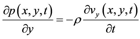
Consider sound waves propagating in the water. Instead of the wave equation, we base our work on the basic Euler’s equation and the equation of continuity. For simplicity, the discussion is confined to a two-dimensional space. In a 2-D Cartesian coordinate system, the sound pressure  and the particle velocity v satisfy the following linear equations:
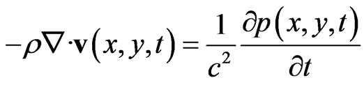 , (1)
, (1)
 , (2)
, (2)
 . (3)
. (3)
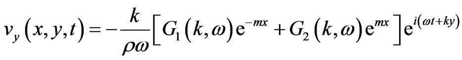
where  is the particle velocity, p(x, y, t) is the pressure and
  is the density of the fluid with wave number
 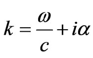 where
where
 ,
,  is the angular frequency, c and
  are the speed of sound and attenuation in inhomogeneous medium, respectively.
3. Normal Mode Analysis
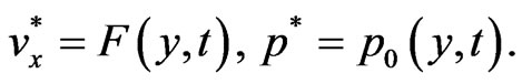
The solution of considered physical variable can be decomposed in terms of normal modes as the following form
 (4)
(4)
where  are the amplitude of the functions
  respectively.
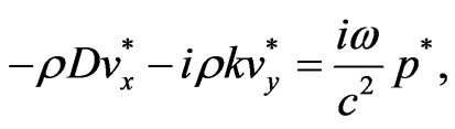
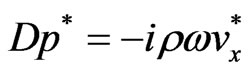
Equations (1)-(3) become
 (5)
(5)
 , (6)
, (6)
 . (7)
. (7)
where, .
.
Equations (5)-(7) form a coupled system Eliminating  and
and  between Equations (5)-(7) we obtain
 (8)
(8)
where, .
.
The solution of Equation (8) has the form
 . (9)
. (9)
where , and
, and  are the roots of the characteristic equation
 (10)
(10)
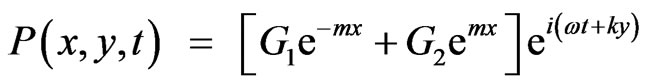
The solution of Equation (8) is given by
 (11)
(11)
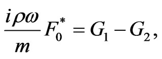
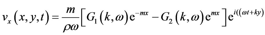
From Equations (6) and (11) we can obtain
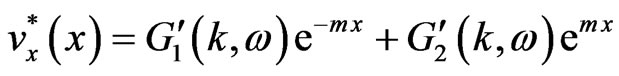 (12)
(12)
where,
 (13)
(13)
From Equations (7) and (11) we can obtain
 (14)
(14)
where,
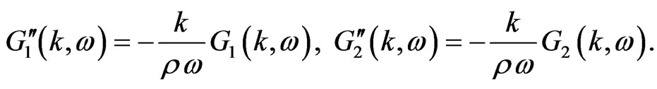 (15)
(15)
4. Boundary Conditions
On the surface at x = 0
 (16)
(16)
Substituting from (4) into (16) then Equations (11) and (14)
 (17)
(17)
 (18)
(18)
By adding Equations (17) and (18) we obtain
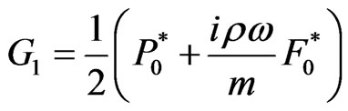 (19)
(19)
By subtracting Equations (17) and (18) we get
 (20)
(20)
By substituting from Equations (19) and (20) into Equations (11), (12) and (14)
 (21)
(21)
 (22)
(22)
 (23)
(23)
5. Computational Results
To study the wave propagation phenomenon in viscous medium and under different frequencies, we can apply the theoretical acoustic viscous wave Equation (21). Using water as the medium, the parameters are given as following:  and
and . Let the wave peak amplitude be
  Pa and
  m/sec at the source (x = 0), we simulate the pressure wave peak amplitude, in Equation (21), vs. the distance from the source at various frequencies. The results are shown in Figure 1 (in dB and linear scale). As expected, the peak wave amplitude becomes smaller as we move further from the source. We can also notice that as the wave frequency goes higher, more attenuation can be observed at any given location. The peak pressure as function of frequency shown in Figure 2 for fixed distance at x = 2 cm. It is clear from this figure that the magnitude of peak of pressure little changes with the frequency. The predicted results are very agreement to the recorded by Wang [14].
Let us consider a 2-D simulation in which the pressure varies in the x and y directions. Figure 3 shows the 2-D pressure computational as function in the plane x-y. From this figure, it can be seen that the pressure amplitude becomes smaller when moving in the x-y plane further from the source.
6. Conclusions
A normal mode analysis which accurately the pressure acoustic wave equation, has been developed. This technique has a number of attractive features, foremost of which is the speed and simplicity with which it can be designed and implemented. The model could be used in
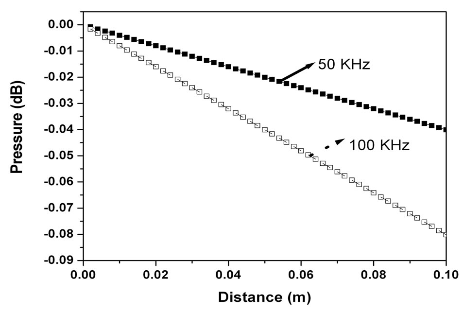
Figure 1. Pressure amplitude (dB) as function of the distance from the origin.
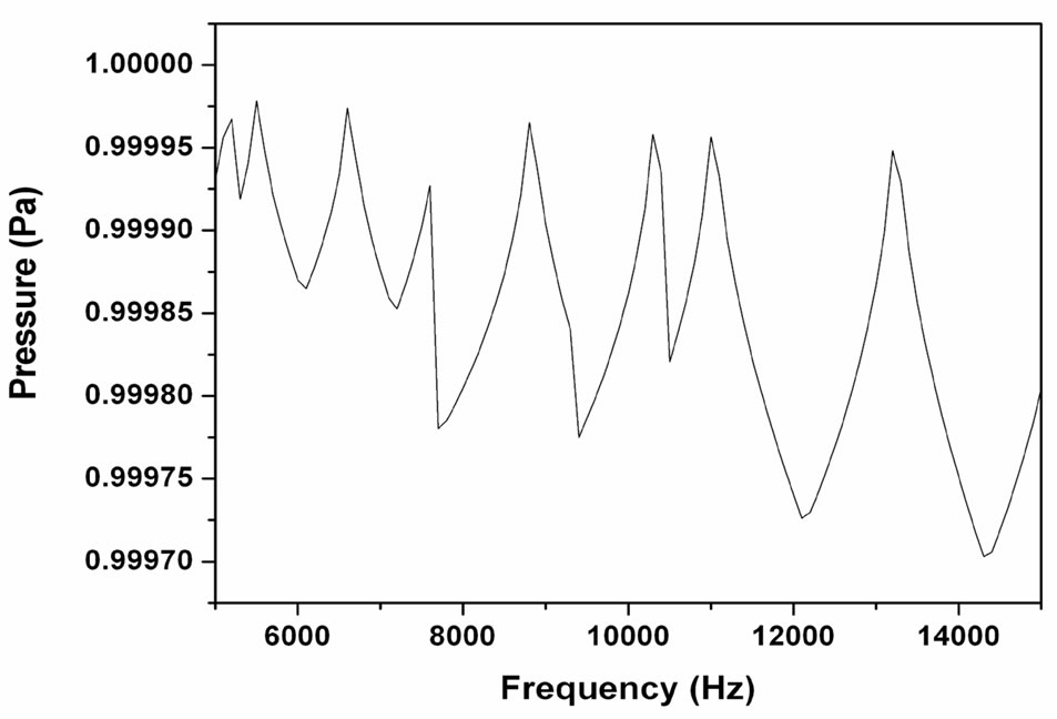
Figure 2. The pressure amplitude as function of frequency at distance 2 cm from the source.
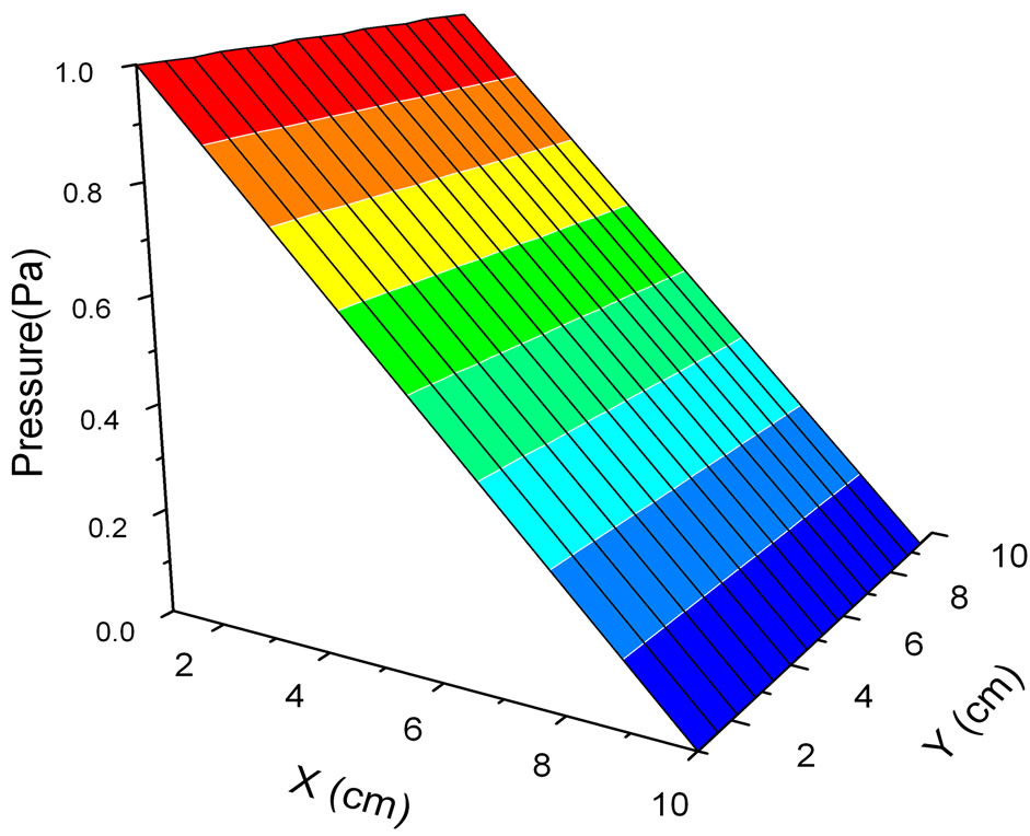
Figure 3. The pressure amplitude as function of plane x-y direction.
the future to incorporate non-linear propagation effects.