Oscillator with Distributed Nonlinear Structure on a Segment of Lossy Transmission Line ()

1. Introduction
The present paper is devoted to investigation of self-oscillators with distributed amplifying structure of tunnel diode type realized on a segment of lossy transmission line. The transmission line is terminated by nonlinear reactive elements. Such problems and their applications (for instance to RF-circuits, PCB-s problems and so on) are usually considered by means of various methods (slowly varying in time and space amplitudes and phases, numerical methods and so on, cf. [1] - [14] ). We have developed (cf. [15] ) a general approach for investigation of lossy transmission lines terminated by nonlinear loads without Heaviside condition . From mathematical point of view in [15] , we consider just linear hyperbolic systems. In [16] and [17] , we have considered a Josephson superconductive transmission line system with sine type nonlinearities. Our main purpose here is to consider lossy transmission line with polynomial nonlinear distributed structure that leads to a nonlinear hyperbolic system. We extend Abolinya- Myshkis method (cf. reference of [16] ) to attack the nonlinear boundary value problem and propose a new general approach to reduce the mixed problem for such nonlinear systems to an operator form in suitable function spaces. The arising nonlinearity is of polynomial type in view of distributed tunnel diode element. The nonlinear characteristics of the reactive elements generate nonlinear boundary conditions. We prove the existence of an approximated solution of the mixed problem and show a way to reach this solution by successive approximations.
We proceed from the circuit shown on Figure 1, where  and
and  are nonlinear reactive elements. We consider that a particular case
  is a nonlinear capacitance, while
  is a nonlinear inductance. In a similar way, it can be treated more complicated circuits (cf. [15] ).
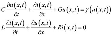
A lossy transmission line with distributed nonlinear resistive element can be prescribed by the following first order nonlinear hyperbolic system of partial differential equations (cf. [1] - [14] ):
 (1)
(1)
![]()
where  and
and  are the unknown voltage and current, while L, C, R and G are inductance, capacitance, resistance and conductance per unit length;
  is itslength; and
  is a prescribed polynomial of arbitrary order with intervalof negative resistance (in the applications most often of third order). For the above
![]()
Figure 1. Lossy transmission line with distributed nonlinear resistive element with an interval of negative differential resistance in the characteristic.
system (1), one can formulate the following initial-boundary (or briefly mixed) problem: to find the unknown functions  and
and  in
in  such that the following initial and boundary conditions are satisfied
 (2)
(2)
 (3)
(3)
where  and
and ![]() are prescribed initial functions the current and voltage at the initial instant;
are prescribed initial functions the current and voltage at the initial instant; ![]() are characteristics of the reactive elements
are characteristics of the reactive elements![]() .
.
Rewrite the system (1) in the form
![]() (4)
(4)
2. Transformation of the Partial Differential System
First we present the system (4) in matrix form:
![]() .
.
Introducing denotations
![]()
![]()
we have
![]() . (5)
. (5)
To transform the matrix ![]() in diagonal form we solve the characteristic equation
in diagonal form we solve the characteristic equation ![]() Its roots are
Its roots are![]() ,
,![]() . The eigen- vectors are
. The eigen- vectors are![]() ,
,![]() . We form the matrix by eigen-vectors
. We form the matrix by eigen-vectors![]() . Then
. Then ![]() and
and ![]() .
.
Introduce new variables![]() , where
, where![]() . Therefore
. Therefore
![]() and
and ![]() (6)
(6)
Substituting ![]() in Equation (5) we obtain
in Equation (5) we obtain
![]()
or
![]() (7)
(7)
But
![]() ,
, ![]()
Then introducing denotations ![]() we obtain from Equation (7)
we obtain from Equation (7)
![]() (8)
(8)
Introduce again new variables
![]() (9)
(9)
and then the system (8) reduces to
![]()
The new transformation formulas are
![]() (10)
(10)
The new initial conditions we obtain from Equations (2), (6) and (9) for![]() :
:
![]()
The new boundary conditions we obtain from Equations (3):
![]() (11)
(11)
In order to solve the last equations with respect to the derivatives we consider the properties of nonlinear capacitive and inductive elements. For the capacitive element (cf. [15] ) we have![]() , where
, where ![]() are constants and
are constants and![]() . If
. If![]() , then
, then ![]() has strictly positive lower bound.
has strictly positive lower bound.
Indeed (cf. [15] ),![]() .
.
To obtain ![]() we make
we make
Assumption (C)![]() .
.
If we choose ![]() it follows
it follows ![]() and
and ![]() for
for ![]() and therefore
and therefore
![]() .
.
Besides
![]() .
.
The inductive element has I-L characteristic of polynomial type.
To solve the second equation (11) with respect to ![]() we make
we make
Assumptions (L)![]() ,
,![]() .
.
In view of ![]() we obtain
we obtain
![]()
![]()
We present the above relations in an integral form under
Assumptions (CC)![]() ,
,
![]()
3. Operator Formulation of the Mixed Problem for the Transmission Line System
Now we are able to formulate the mixed problem with respect to the unknown functions![]() : to find
: to find ![]() satisfying the system and initial and boundary conditions
satisfying the system and initial and boundary conditions
![]()
(12)
In what follows we give an operator representation of the above mixed problem (12).
Recall that ![]() and
and ![]() and
and![]() . The ordinary differential equations (Cauchy problem) for the characteristics of the hyperbolic system are
. The ordinary differential equations (Cauchy problem) for the characteristics of the hyperbolic system are
![]() for each
for each ![]() (13)
(13)
![]() for each
for each ![]() (14)
(14)
The functions ![]() and
and ![]() are continuous ones. This im- plies that for every
are continuous ones. This im- plies that for every ![]() there is a unique (to the left from
there is a unique (to the left from![]() ) solu- tion
) solu- tion ![]() for
for![]() ;
;![]() , and respectively
, and respectively ![]() for
for![]() ;
;![]() . Denote by
. Denote by ![]() the smallest value of
the smallest value of ![]() such that the solution
such that the solution ![]() of Equation (13) still belongs to
of Equation (13) still belongs to ![]() and respective-
and respective-
ly the solution ![]() of Equation (14) by
of Equation (14) by![]() . If
. If ![]() then
then ![]() or
or ![]() and respectively if
and respectively if ![]() then
then ![]() or
or![]() . In our case
. In our case
![]() ;
; ![]()
Remark 1. We notice that![]() . It is easy to see that
. It is easy to see that
![]()
![]()
Introduce the sets:
![]()
![]()
![]()
![]()
![]()
![]() .
.
Prior to present problem (12) in operator form we introduce
![]()
and
![]()
or
![]()
![]()
So we assign to the above mixed problem the following system of operator equations (cf. [16] , [17] ):
![]()
![]()
4. Existence Theorem
In order to obtain a contractive operator we consider the mixed problem (12) on the subset![]() . We introduce the sets
. We introduce the sets
![]() and
and ![]()
where ![]() and μ are positive constants chosen below. It is easy to verify that
and μ are positive constants chosen below. It is easy to verify that ![]() turns out into a complete metric space with respect to the metric
turns out into a complete metric space with respect to the metric
![]() ,
,
where
![]() ,
,
![]() .
.
Now we define an operator ![]() by the formulas
by the formulas
![]()
![]()
Remark 2. Assumption (C) and Assumptions (L) in view of Equations (10) imply
![]() ;
;![]() .
.
Theorem 1. Let the following conditions be fulfilled:
1) Assumption (C), Assumptions (L), Assumption (CC) and![]() ,
, ![]() for
for ![]() as
as ![]() are sufficiently small while
are sufficiently small while ![]() is sufficiently large;
is sufficiently large;
2)![]() ;
;
3)![]() ;
;
4)![]() ;
;
5)![]() .
.
Then there exists a unique solution of the problem (12).
Proof: We establish that the operator B maps the set ![]() into itself.
into itself.
First we notice that ![]() and
and ![]() are continuous functions. We show
are continuous functions. We show
![]() ,
,![]() .
.
Indeed, for sufficiently small ![]() and in view of
and in view of ![]() and
and ![]() we have
we have
![]()
Then for the first component we have
![]()
In view of
![]()
and
![]()
for sufficiently small ![]() for the second component we obtain:
for the second component we obtain:
![]()
Now we show that B is a contractive operator.
Indeed, for the first component we obtain:
![]()
Similarly for the second component we obtain
![]()
Therefore
![]()
and the operator B has a unique fixed point which is a solution of the mixed problem above formulated in the set![]() .
.
Theorem 1 is thus proved.
Remark 3. We point out that for every ![]() there is a unique solution
there is a unique solution ![]() in
in![]() . The sequence
. The sequence ![]() is not necessary convergent when
is not necessary convergent when![]() . To find a convergent subsequence we proceed as in [17] . Extending the solution on
. To find a convergent subsequence we proceed as in [17] . Extending the solution on ![]() we can choose a convergent subsequence. The first approximation can be chosen, for instance, as a solution of the linearized system (12).
we can choose a convergent subsequence. The first approximation can be chosen, for instance, as a solution of the linearized system (12).
5. Conclusion Remarks
1) We note that the interval ![]() is not sufficiently small.
is not sufficiently small.
2) We show a simple verification of all inequalities of the main theorem for soft nonlinearity ![]() (cf. [1] ). Consider a lossy transmission line (cf. [1] - [15] ) satisfying the Heaviside condition with specific parameters:
(cf. [1] ). Consider a lossy transmission line (cf. [1] - [15] ) satisfying the Heaviside condition with specific parameters:
![]() ;
;
![]() ;
;![]() ;
;
![]() ;
;
![]() ;
;
![]() .
.
Let us choose a polynomial ![]() with interval of negative differential resistance,
with interval of negative differential resistance, ![]() and
and![]() . Then
. Then![]() ;
; ![]() . The pn-junction capacity is
. The pn-junction capacity is ![]() , while the pn-junction potential
, while the pn-junction potential![]() . For
. For ![]() and
and ![]() the minimal value of
the minimal value of ![]() is
is![]() .
.
We choose ![]() such that
such that![]() .
.
Then the inequalities from Remark 3 and two of inequalities from Theorem 1 become
![]() ;
;
![]()