Explicit Solutions of the Coupled mKdV Equation by the Dressing Method via Local Riemann-Hilbert Problem ()
1. Introduction
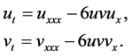
The coupled mKdV equation
 (1)
(1)
In this paper, we study the Equation (1) with the help of the Riemann-Hilbert method following [15] [16] . The present paper is organized as follows. In section 2, we give the Jost solution of the spectral equation. In section 3, we discuss the analytic property of the Jost solution. In section 4, we give the Matrix Riemann-Hilbert Problem. In section 5, we obtain the soliton-solution of the coupled KdV Equation (2), and we drop the curve of the solutions with the aid of the Matlab.
2. Jost Solution
First, we consider the coupled KdV equation
 (2)
(2)
As is well known [2] , the Equation (2) can be derived as the compatibility of the system
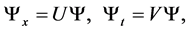 (3)
(3)
where the 2 × 2 matrices U and V of the form
 (4)
(4)
 (5)
(5)
where k is an arbitrary constant spectral parameter.
When , we obtain the special solution of Equation (3). For convenience, we denote the special solution as
 . Then, the spectral Equation (3) is transformed into
 (6)
(6)
where, .
.
In what follows, we study the Jost solutions  of the Equation (6) satisfying the asymptotic conditions
 , at
, at . Since
 , these boundary conditions guarantee that
  for all x.
In fact, the Jost functions  are not mutually independent. They are interconnected by the scattering matrix
 :
:
 (7)
(7)
3. Analysis Solutions
Let us rewrite the spectral Equation (6) with the boundary conditions in the integral form:
 (8)
(8)
for the first column entries of the Jost matrix![]() .
.
It is easy to know that the exponent in (8) decreases for![]() . The first column
. The first column ![]() of the matrix
of the matrix ![]() is analytic in the upper half plane and continuous on the real axis
is analytic in the upper half plane and continuous on the real axis![]() . Similarly, we know that the second column
. Similarly, we know that the second column ![]() of the matrix
of the matrix ![]() is analytic as well in the same domain. Then, we give a solution of Equation (6):
is analytic as well in the same domain. Then, we give a solution of Equation (6):
![]()
It can see that it is analytic as a whole in the upper half plane.
The analytic solution ![]() can be expressed in terms of the Jost function. In view of (7), we derive
can be expressed in terms of the Jost function. In view of (7), we derive
![]() (9)
(9)
with
![]() (10)
(10)
In the same way,
![]() (11)
(11)
It follows from the above formal as that
![]() (12)
(12)
In what follows, we define a function![]() . It is obvious that
. It is obvious that
![]()
Then, ![]() is a solution of the adjoint spectral problem. On the real axis
is a solution of the adjoint spectral problem. On the real axis
![]()
and![]() ,
, ![]() has an asymptotic expansion as follows:
has an asymptotic expansion as follows:
![]() (13)
(13)
and substitute it into the spectral Equation (6). Comparing with powers of k, we derive
![]() (14)
(14)
In order to solve the coupled KdV Equation (2), we should find the analytic solution![]() .
.
4. Matrix RH Problem
Through tedious calculation, we obtain RH problem
![]() (15)
(15)
with![]() ,
,![]() .
.
It is easy to know that ![]() only depends on k, the x-dependence being given by the simple exponential function F. Moreover, it is obvious that
only depends on k, the x-dependence being given by the simple exponential function F. Moreover, it is obvious that ![]() for
for![]() , in view of (12).
, in view of (12).
In order to obtain the soliton solution of the coupled KdV equation, we suppose that the zeros of ![]() and
and ![]() are simple and finite number. We know that determinants of the matrices
are simple and finite number. We know that determinants of the matrices ![]() and
and ![]() are given by
are given by ![]() and
and![]() . We assume that
. We assume that
![]()
![]()
In this case, the RH problem (15) with zeros can be solved in view of its regulation.
To obtain the relevant regular problem, let us introduce a rational matrix function
![]()
where the eigenvector ![]() solves
solves![]() .
.
Here ![]() is the rank 1 projector
is the rank 1 projector![]() , and
, and![]() .
.
In view of (11), we know that ![]() near the point
near the point![]() . We obtain
. We obtain ![]() at the point
at the point![]() . The matrix function
. The matrix function ![]() will be regularized by the rational function
will be regularized by the rational function
![]()
it is easy to know that the matrix ![]() has no zeros in
has no zeros in![]() .
.
The regularization of all the other zeros is performed similarly, and eventually we obtain the following representation for the analytic solutions:
![]() (16)
(16)
where the rational matrix function ![]() accumulates all zeros of the RH problem, while the matrix functions
accumulates all zeros of the RH problem, while the matrix functions ![]() solve the regular RH problem (without zeros)
solve the regular RH problem (without zeros)
![]() (17)
(17)
with![]() , thus
, thus![]() .
.
The matrix ![]() will be called the dressing factor. It follows from (16) that the asymptotic expansion for the dressing factor is written as
will be called the dressing factor. It follows from (16) that the asymptotic expansion for the dressing factor is written as
![]() (18)
(18)
We note that the dress matrix ![]() can be written as
can be written as
![]()
![]() (19)
(19)
![]() (20)
(20)
Thus, we derived ![]() vectors
vectors ![]() and
and ![]() instead of N vectors
instead of N vectors![]() . It is obvious that
. It is obvious that ![]() at the point
at the point![]() . To avoid divergence at
. To avoid divergence at![]() , we should pose
, we should pose![]() , that is
, that is
![]() (21)
(21)
We note that the matrix ![]() can be decomposed into the following form:
can be decomposed into the following form:
![]() (22)
(22)
where![]() . Similarly,
. Similarly,
![]() (23)
(23)
where![]() . In what follows, we rewrite (13) as
. In what follows, we rewrite (13) as
![]() (24)
(24)
Let us differentiate the equation ![]() in x, and in view of (6), we derive
in x, and in view of (6), we derive
![]()
thus, we have
![]() (25)
(25)
In the same way, we obtain the evolutionary equation
![]() (26)
(26)
In this end, we establish explicitly the vector ![]() as
as
![]() (27)
(27)
where ![]() is a vector integration constant.
is a vector integration constant.
Similarly, according to![]() , we obtain the solution
, we obtain the solution
![]() (28)
(28)
where ![]() is a vector integration constant.
is a vector integration constant.
5. One Soliton Solution
We consider the case ![]() and pose
and pose![]() ,
,![]() . Then, we have
. Then, we have
![]() (29)
(29)
where, ![]() are components of the constant vector
are components of the constant vector![]() .
.
![]() (30)
(30)
where, ![]() are components of the constant vector
are components of the constant vector![]() .
.
The dress formula (19) reduced to
![]() (31)
(31)
At the same time, we have![]() , from which, we obtain
, from which, we obtain
![]() . (32)
. (32)
Denoting![]() ,
, ![]() , thus
, thus
![]() (33)
(33)
In the same way, defining![]() ,
, ![]() , thus
, thus
![]() (34)
(34)
Substituting (31) and (32) into (30), we have
![]()
Moreover, ![]() , hence,
, hence,
![]()
From which, we have the solutions of the coupled KdV Equation (2)
![]() (35)
(35)
Here, ![]() ,
, ![]() ,
, ![]() and
and ![]() determine the soliton velocity and amplitude, respectively, while
determine the soliton velocity and amplitude, respectively, while![]() ,
, ![]() ,
, ![]() and
and ![]() give the initial position and phase of the soliton. In what follows, we plot the graph for
give the initial position and phase of the soliton. In what follows, we plot the graph for ![]() in order to analyze the solutions (35). Figure 1 and Figure 2 are the imaginary part and real part of
in order to analyze the solutions (35). Figure 1 and Figure 2 are the imaginary part and real part of![]() , respectively. From the two solution curves, we can see that the difference between the real and imaginary part.
, respectively. From the two solution curves, we can see that the difference between the real and imaginary part.
In the same way, we drop the solution curves of v for Figure 3 and Figure 4.
From the graphs, it is shown that u and v have the similar solution form. The difference exists between the real and imaginary part. In fact, we chose different parameters, and the solution curves between the real part and imaginary part had corresponding changes.
Acknowledgements
The authors acknowledge the support by National Natural Science Foundation of China (Project No: 11301149), Henan Natural Science Foundation For Basic Research under Grant No: 162300410072, doctor Foundation (D2015001) and Young backbone teachers in Henan province.