Gedanken Experiment (Thought Experiment) about Gravo-Electric and Gravo-Magnetic Fields, and the Link to Gravitons and Gravitational Waves in the Early Universe ()
Received 4 November 2015; accepted 24 April 2016; published 27 April 2016

1. Introduction
Reviewing What Was Done by Padmanabhan as Far as Gravo-Electromagnetic Waves Being Set up So as to Have up for Calculation of Using the Results of Initial Energy as Due to 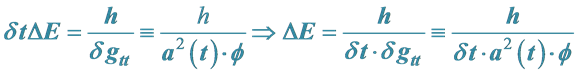 and Comparing It to a More General Energy Expression Given below
Our tack is to take what is given by the energy expression from [1] , with an minimum energy given as, if  is an inflaton, and if
  is the square of the scale factor, and
  a non-dimensional perturbation of the “time” factor in a geodestic, that then by [1] [2]
 (1)
(1)
And then what we do is to take the work from [3] to come up with a gravo-electromagnetic frequency which is then set as equal to give an initial import of energy according to a frequency
 (2)
(2)
This frequency, as isolated in Equation (2) will be compared to the frequency generated by the gravo-electric and gravo-magnetic fields given in the following argument below. It will suggest something about the inflaton, as suggested in the last part of this document.
We will take the square of the frequency given in the 2nd line of Equation (2) and compare it to gravo-electric and gravo-magnetic generated frequency value, as our first principle linkage of electromagnetic waves with gravitons. We should keep in mind that the volume, which is for a complete cosmology is small.
So, let us now come up with a gravo-electric & gravo-magnetic counterpart to Equation (2) above. To do that, we take an argument given in [3] in pages 278 - 279 of the form , from exercise 6.15 of a magnetic and electric field being generated by a source with arbitrary density, as to have the following two lowest order perturbations,
as given in the exercise to be, if M is total mass,  the angular momentum tensor with also
  a momentum density defined by
 , to yield the gravo-electric tensor
 , and gravo-mag- netic potential
 . Then, we shall reference the potential’s given below. Note, that we are referring to a
volume, V, which will be for the entire spatial domain of the universe but that our V volume is in early universe conditions of Planckian size dimensions. The author thanks the referee for the necessity of making this point obvious as how to properly interpret Equation (1) given above. Here, G is the usual gravitational “constant”, c the speed of light, and what is called x is the spatial dimensions.  as the angular momentum tensor should be thought of in terms of, in this case, as having a relationship to electromagnetics, as given in [4] below whereas
 (3)
(3)
we are taking Equation (1) as formulated from equations from pages 278-279 of the text as given in reference [3]
Then again by [3] , and exercise 6.15, page 279, the following gravo-electric and gravo-magnetic fields appear
 (4)
(4)
Here,  is a unit vector in the radial direction, and
 ![]() an angular velocity, which will then lead to the following angular frequency, that by [3] , and exercise 6.15, page 279
an angular velocity, which will then lead to the following angular frequency, that by [3] , and exercise 6.15, page 279
![]() (5)
(5)
From here, we will proceed to modify M, and ![]() by gravitational physics.
by gravitational physics.
2. Modify M, and S by Gravitational Physics
What we are going to do, is the restrict M to the case of heavy gravity in the Planckian regime, call G the usual gravitational physics variable, and define S, as following for M and S. N being the number of initial gravitons, and a radii as Planck length![]() , with
, with ![]() > 0, so up to a good approximation
> 0, so up to a good approximation
![]() (6)
(6)
Then the maximum initial value of the angular frequency of Equation (5) is
![]() (7)
(7)
3. Modify M, and S by Gravitational Physics with Numerical Inputs into Equation (7) for Frequency
![]() , due to and a rest massive graviton mass of about 10^−62 grams, due to [5] plus a radial distance r from the source of the graviton production would lead to relic gravitational waves reduced dramatically from the beginning radii presumably about 1 meter, to the present radii of the universe, presumably of the value of about
, due to and a rest massive graviton mass of about 10^−62 grams, due to [5] plus a radial distance r from the source of the graviton production would lead to relic gravitational waves reduced dramatically from the beginning radii presumably about 1 meter, to the present radii of the universe, presumably of the value of about![]() .
.
If so, then, the energy would be represented, if ![]() and we have by [6]
and we have by [6]
![]() (8)
(8)
Then from [4] [6] we have for gravitons an energy value of about, if m is the mass of a “massive” graviton, using in this case the relativistic formula as given in [2] [6] , to approximate to first order
![]() (9)
(9)
Compare this value of energy, by making the following scaling, namely equate Equation (5) and Equation (9) such that
![]() (10)
(10)
Which is then compared with and is implying a frequency squared value of [2]
![]() (11)
(11)
To get to the present value of what the relic wavelengthfor produced gravitons initially would be, take in the upper value of the ![]() given in Equation (11) that
given in Equation (11) that![]() , as in [5] would be if r in Equation (10) is
, as in [5] would be if r in Equation (10) is ![]()
![]() (12)
(12)
Whereas if r in Equation (10) is significantly less than 1 meter, emergent radiation would be
![]() (13)
(13)
Based upon Equation (12) and Equation (13)
![]() (14)
(14)
This is using extremely rough estimates.
4. Considerations as to Bicep 2, the Matter of Scalar-Tensor Polarizations as an Alternative to General Relativity and Alternate Gravitational Theories and Experimental Tests of General Relativity via Inteferometric Methods
From [7] we have the following to consider, namely trying to determine restraints upon the nature of gravity, i.e. is it consistent with General relativity or do we have an alternative situation as given in the following quote. We hope that getting a consistent model of inflaton physics will help clarify the following alternatives:
Quote
This fact rules out the possibility of treating gravitation like other quantum theories, and precludes the unification of gravity with other interactions. At the present time, it is not possible to realize a consistent Quantum Gravity Theory which leads to the unification of gravitation with the other forces. On the other hand, one can define Extended Theories of Gravity those semiclassical theories where the Lagrangian is modified, in respect to the standard Einstein-Hilbert gravitational Lagrangian, adding high-order terms in the curvature invariants (terms like R2, etc…) or terms with scalar fields non minimally coupled to geometry (terms like φ2R)
End of quote
We claim that the strength of the inflaton term , as we will give in Equation (15) may allow us to determine if we have to use a semi classical set of terms which add more terms to the space curvature of early universe Planckian physics space time geometry. We also though have to temper this quest in requiring that the following holds as given in [8] , namely:
Quote
Recent data from Planck matches well with the minimal ΛCDM model. A likelihood analysis using Planck, WMAP and a selection of high resolution experiments (highL), tensor to scalar ratio r 0.002 is found to be <0.11 when dns/dlnk = 0.
End of quote
Our inflaton, which is given in Equation (15) must be made consistent with the requirements of a low scalar to tensor ratio, and this requires exquisite fine tuning of inputs into the inflaton, which also should be made consistent with answers to [7] - [9] .
We find that the resulting inflaton measurement which is the conclusion of our document, with the following, namely assuming that![]() , and which may involve [10] directly. I.e. is our inflaton con-
, and which may involve [10] directly. I.e. is our inflaton con-
sistent with just two standard polarizations, or is there a third polarization necessary so that the following inflaton forms? If there is not a response function of an interferometer to an additional “scalar” polarization we define, we stick to GR, whereas though if Equation (15) necessitates an additional polarization, we are looking at a scalar-tensor gravitational theory. Needless to say we will require careful analysis of
![]() (15)
(15)
5. Avoiding the Bicep 2 Mistake: What We Can Do with Equation (15)?
Following [9] what we are doing is examining the stochastic regime of space-time where the following holds:
Quote
Omni-directional gravitational wave background radiation can arise from fundamental processes in the early Universe, or from the superposition of a large number of signals with a point-like origin. Examples of the former include parametric amplification of gravitational vacuum fluctuations during the inflationary era, termination of inflation through axion decay or resonant preheating, Pre-Big Bang models inspired by string theory, and phase transitions in the early Universe; the observation of a primordial background will give access to energy scales of 10 to the 9 power, up to 10 to the 10 power GeV, well beyond the reach of particle accelerators on Earth.
End of quote
Needless to say though, we need above all to avoid getting many multiple stochastic signals, in what we process for primordial gravitational waves, and to use, instead tests to avoid getting dust signals which are what doomed Bicep 2, i.e. as is made very clear in [12] [13] . In all, what we are doing is consistent with the requirements given in the Authors other article, [14] , as is given in the following quote:
Quote
The main agenda will be in utilization of Equation (27) to help nail down a range of admissible frequencies which will be to avoid [11] - [14] conflating the frequencies of collected gravitational wave signals from relic cosmological conditions (or would be signals) with those connected with dust generated gravitational wave signals, especially from dust conflated with Galaxy formation in the early universe. More than anything else, we need to find likely narrow (?) Frequency ranges, which will be commensurate with Equation (27), and to use advanced detector technology. Of course such a search will be hard. But it also will be a way, with due diligence as to answer questions raised by the Author in [14] . In doing so, the relative flatness of the early universe and its departure from curved space conditions will be a great way to answer the suppositions raised in [9] [10] as well.
End of quote
Understanding inflaton physics properly will also give credence to considerations given in [1] below as to the degree of flatness or lack of, in the early Universe.
Acknowledgements
This work is supported in part by National Nature Science Foundation of China grant No. 11375279.