Optimal Investment and Risk Control Strategy for an Insurer under the Framework of Expected Logarithmic Utility

Tingyun Wang

Department of Statistics, Jinan University, Guangzhou, China.

DOI: 10.4236/ojs.2016.62024                

Abstract

In this paper, we consider an insurer who wants to maximize its expected utility of terminal wealth by selecting optimal investment and risk control strategies. The insurer’s risk process is modeled by a jump-diffusion process and is negatively correlated with the returns of securities and derivatives in the financial market. In the financial model, a part of insurers’ wealth is invested into the financial market. Using a martingale approach, we obtain an explicit solution of optimal strategy for the insurer under logarithmic utility function.

Keywords

Jump-Diffusion Process, Logarithmic Utility, Martingale Approach

Received 2 March 2016; accepted 23 April 2016; published 26 April 2016

1. Introduction

In the past two decades, more and more attention has been paid to the problem of optimal investment in financial markets for an insurer. Indeed, this is a very important portfolio selection problem for the insurer from a point of finance theory. Merton (1969) [1] first used stochastic control theory to solve consumption and investment problem in framework of continuous financial market. Based on the Merton’s work, Zhou and Yin (2004) [2] , and Sotomayor and Cadenillas (2009) [3] considered consumption/investment problem in a financial market with regime switching. Under the mean-variance criterion and the utility maximization criterion, respectively, they obtained explicit solutions. In view of an external risk which can be insured against by purchasing insurance policy into Merton’s framework, Moore and Young (2006) [4] cooperated and studied optimal consumption, investment and insurance problem. Following Moore and Young (2006) [4] , Perera (2010) [5] resolved the same problem in a more general Levy market. Along the same work, many researchers applied an uncontrollable risk process to Merton’s model, such as Yang and Zhang (2005) [6] . They considered stochastic control problem for optimal investment strategy without consumption under a certain criteria.

For an insurer, since reinsurance is an important tool to manage its risk exposure, optimal reinsurance problem should be considered carefully. This issue implies that the insurer has to select reinsurance payout for certain financial objectives. The classical model for risk in the insurance literatures is Cramer-Lundberg model, which uses a compound Poisson process to measure risk. Based on the limiting process of compound Poisson process, Taksar (2000) [7] wrote the paper about optimal risk and dividend distribution control. Following his same vein, recent researches started to model the risk by diffusion process or a jump-diffusion process; see, e.g. Wang (2007) [8] and Zou (2014) [9] . Considering both proportional reinsurance and step-loss reinsurance, Kaluszka (2001) [10] researched optimal reinsurance in discrete time under the mea-variance criterion. What’s more, recent generalizations in modeling optimal reinsurance process include incorporating regime switching, and interest rate risk and inflation risk; see Zhuo et al. (2013) [11] Guan and Liang (2014) [12] respectively.

In this paper, the model and optimization problem are different from others. Firstly, it is not total wealth of insurer invested, but a part of wealth invested. So in this model, we can obtain the optimal property of the total wealth. Secondly, different from Merton’s work, we use a jump-diffusion process to model an insurer’s risk. Lastly, we regulate the insurer’s risk by controlling the number of polices.

This paper is organized as follow. In Section 2, we formulate investment and risk control problem and describe the financial model and risk process model. The explicit solution of optimal investment and risk control strategy for logarithmic utility is derived in Section 3. In Section 4, we conduct a sensitive analysis. Conclusions of the research are reached in Section 5.

2. The Financial Model and the Risk Process Model

Suppose that there are two assets for investment in the financial market. One is a riskless asset with price process and the other is a risky asset with price process. The dynamic of and are give by

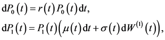(2.1)

respectively, where and are positive bounded functions and is a standard Brownian motion. The initial conditions are and

For an insurer, most of its incomes come from writing insurance policies, and we denote the total outstanding number of policies at time t by. To simplify our analysis, we assume that the insurer’s average premium for per policy is p, so the total incomes from selling insurance policies over the time period is given by

A classical risk model for claims is compound Poisson model, in which the claim for per policy is given by where is a series of independent and identically distributed random variables, and is a Poisson process independent of. If the mean of and the intensity of are finite, such compound Poisson process is a Levy process with finite Levy measure. According to Oksendal and Sulem (2005, Theorem 1.7) [13] , a Levy process can be decomposed into three components, a linear drift part, a Brownian motion part and a pure jump part. Based on this theorem, we suppose the insurer’s risk for per policy is given by

(2.2)

where is a standard Brownian motion and N is a Poisson process defined on the given filtered space, respectively. We assume that are all positive constants. As Stein (2012) [14] considered, we assume

(2.3)

where and is another standard Brownian motion, independent of. We also suppose that the Poisson process N has a constant intensity, and is independent of both and.

For an insurer, it should be noted that it is impossible for an insurer to invest its total wealth. At time t, we denote as a part of the insurance wealth invested. Under this consideration, we let and be the amount invested in the risky asset and the total liabilities respectively. For a strategy the terminal wealth process is driven by the following SDE:

(2.4)

with initial wealth

Following Stein (2012, chapter 6) [14] , we define the liability radio of liabilities over surplus as . We denote as the total proportion of wealth invested, as the proportion of wealth invested in the risky asset at time t. Then for a control, we have. Then we can rewrite SDE (2.4) as

(2.5)

with initial wealth.

In this model, as Zou (2014) [9] considered, to compensate extra risk by extra return, the coefficients must satisfy the following conditions: and.

Define the criterion function as, where is the terminal time, and is a

conditional expectation under probability measure P given. The utility function U is assumed to be a strictly increasing and concave. In this paper, the choice for the utility function in economics and finance is. We denote as the set of all admissible controls with initial wealth. In Section 3, we give the formal definition of when and choose either u or to be a control. The value function is defined by

(2.6)

where u will be changed accordingly if the control we choose is.

3. The Analysis for

Firstly formulate the stochastic control problem. The problem in this model is to select an admissible control (or) that attains the value function. The control (or) is called an optimal control or an optimal policy. We choose u as an admissible control and for every is progressively measurable and satisfies the following conditions,

. (3.1)

Furthermore, we assume while to avoid the possibility of bankruptcy at jumps.

As we know that for, the SDE (2.5) satisfies the linear growth condition and Lipschitz continuity condition, thus by Theorem 1.19 in Oksendal and Sulem (2005) [13] , there exists a unique solution such

that for all

Applying Ito’s formula to, we can obtain that

(3.2)

where is the compensated Poisson process of N and is a martingale under P. Let

(3.3)

Proposition 3.1. The associated optimal terminal wealth is strictly positive with probability 1 under optimal control.

Proof. According to (2.5) and the Doleans-Dade exponential formula, we have that

(3.4)

From (3.4), to prove with probability 1, we just need to prove with probabili-

ty 1. For any, and or 0, we have So we can obtain that

. This implies that with probability 1.

Next, we will use the martingale method to get an optimal control for the SDE (2.5). To begin with, we give two important Lemmas. Lemma 3.1 gives the condition that optimal control must satisfy while Lemma 3.2 is a generalized version of martingale representation theorem.

Lemma 3.1. (Wang (2007) [8] ) If there exists a control such that is con-

stant over all admissible controls, then is optimal control.

Lemma 3.2. (Wang (2007) [8] ) There exists a predicable process for any P-martingale Z such that for all

for all. (3.5)

Now for the value function we obtain optimal control by 3 steps.

Step 1: Conjecture candidates for optimal control.

Following the definition in Zou (2014) [9] , we also define that

and (3.6)

for any stopping time almost surely. According to the Proposition 3.1, the process Z is a strictly positive and square-integral martingale under P with, for all. Define a new measure Q by.

From the SDE (2.4), we have

(3.7)

From the above expression of X and Lemma 3.1, for all admissible strategies, we have

(3.8)

is constant.

Define. Since Z is a P-martingale, so is C.

According to Lemma 3.2, there exists a predictable process such that

(3.9)

From the Doleans-Dade exponential formula, we can obtain that

(3.10)

Through Girsanov’s Theorem, is a Brownian motion under Q and

is a martingale under Q.

For a stopping time let, that is and,which is an admissible

control. By substituting this control into (3.8), we have is a constant for all

which implies that is a Q-martingale.

So must satisfy the equation that

(3.11)

Let and. By a similar way as above, we have

(3.12)

is a Q-martingale, which in turn yields that

(3.13)

From the SDE (2.5), we can derive to,

(3.14)

Comparing the and terms in (3.10) with (3.14), we obtain that

(3.15)

By substituting (3.15) into (3.11) and (3.13), we have that

(3.16)

(3.17)

which the coefficients define as

(3.18)

With the conditions above, solve the Equation (3.17) to get. Since,

, (3.19)

where

According to the (3.19), we can derive with (3.16).

Then we choose that and to get. Similarly, by substituting this control into (3.8), we have

(3.20)

so we can have by the Equation (3.20).

Step 2: Verify that Z_T defined by (3.10) is consistent with its definition, for given in (3.15) and

defined by (3.16), (3.17) and (3.20).

First rewrite (3.14) as

(3.21)

where

(3.22)

Then substituting (3.15) back into (3.10), we can obtain where

(3.23)

is constant.

According to the (3.6), Z is a P-martingale and, then. Therefore,

(3.24)

so Z given by (3.10) with provided by (3.15) is the same as the definition in (3.6).

Step 3: Prove that satisfies the Lemma 3.1.

For any, we give a definition for a new process as follows

(3.25)

From the Equation (3.13), the above issue will be 0, and then the process is a local martingale. As

is a deterministic and bounded, Z is a square-integral martingale under P, that is to say. Meantime, for all, we can obtain that, so is. Therefore, we can derive

, (3.26)

which make possible for us to conclude that the family is uniformly integral under Q for any stopping time. Thus is indeed a martingale under Q with for any. So we can prove that Lemma 3.1 is satisfied. Therefore, we have an optimal control for the function.

4. Sensitive Analysis

In this part, we analyze the influence of the market parameters on the optimal control. To simplify the analysis, we assume that the coefficients are constant in the financial market and the parameters are given in Table 1 which was also used in Zou (2014) [9] . From Table 1, we know that the variables and are not fixed, so we shall analyze the impact of and on the optimal control.

Firstly, we fix to research the influence of. The optimal control of are given by (3.16), (3.17), (3.20), respectively. We draw the graph of optimal control with different values of in Figure 1. From Figure 1, we can know that optimal investment proportion in the securities is an increasing function of, and the optimal liability ratio is like a convex function of. Besides, the optimal total proportion of wealth invested is decreasing when and then increasing. What’s more, the graph shows that. The reason for this behavior comes from the equations of R and in (2.2). For our parameters, there is much uncertainty in the insurance market when belongs to the interval, and hence takes a minimum value in that interval. While takes value near 0 there is little uncertainty, so takes a maximum value. Since is calculated from the equation (3.16), also takes a maximum value when takes value near 0.

Secondly, we fix to analyze the impact of. Consider which include the previous situation. We have a graph of optimal control with different value of in Figure 2. Figure 2 shows that the optimal investment proportion in the securities is an increasing function of, and the optimal total proportion of wealth invested and the optimal liability ratio are both decreasing function of. This situation is supported by the economic interpretation of. In this model, the greater, the more risk for insurers. So, when rises, a risk averse insurer reduces its optimal liability ratio. As the optimal investment expressions (3.17), we know that when raises, increases as well. Besides, according to the optimal total proportion of wealth invested and the optimal liability ratio expressions (3.20) and (3.17) respectively, we know that when rises, and decreases however.

Table 1. Market parameters.

Figure 1. Impact of on the optimal control.

Figure 2. Impact of on the optimal control.

5. Conclusions

In our model, the insurer’s risk process obeys a jump-diffusion process, and it is not total its capital to invest but a part of wealth to invest in financial market. Besides, we consider that an insurer wants to maximize its expected utility of terminal wealth by selecting optimal control. According to the sensitive analysis, we know that the optimal total proportion of wealth invested and the optimal liability ratio are convex functions of, but they are both decreasing functions of. The optimal investment proportion in the securities or derivatives is an increasing function for both and, and. Furthermore, we find that the higher risk insurers get, the lower liability ratio insurers select.

The limitation in this paper is that the liability is an average for per policy, which conflicts with the fact that the premium for per policy changes all the time for different insurance. Therefore we can research the liability described with a linear function in the model. Besides, the model proposed in the paper can be further explored in another ways as well, something we plan to do in future work.

Acknowledgments

The author thanks to the editor and the reviewers for their thoughtful comments that help the author improve a prior version of this article.

Conflicts of Interest

The authors declare no conflicts of interest.

References

[1]	Merton, R. (1969) Lifetime Portfolio Selection under Uncertainty: The Continuous Time Case. Review of Economics and Statistics, 51, 227-257. http://dx.doi.org/10.2307/1926560
[2]	Zhou, X.Y. and Yin, G. (2004) Markowitz’s Mean-Variance Portfolio Selection with Regime Switching: A Continuous-Time Model. SIAM Journal on Control and Optimization, 42, 1466-1482. http://dx.doi.org/10.1137/S0363012902405583
[3]	Sotomayor, L. and Cadenillas, A. (2009) Explicit Solutions of Consumption Investment Problems in Financial Market with Regime Switching. Mathematical Finance, 19, 251-279. http://dx.doi.org/10.1111/j.1467-9965.2009.00366.x
[4]	Moore, K. and Young, V. (2006) Optimal Insurance in a Continuous-Time Model. Insurance: Mathematics and Economics, 39, 47-48. http://dx.doi.org/10.1016/j.insmatheco.2006.01.009
[5]	Perera, R. (2010) Optimal Consumption, Investment and Insurance with Insurable Risk for an Investor in a Levy Market. Insurance: Mathematics and Economics, 46, 479-484. http://dx.doi.org/10.1016/j.insmatheco.2010.01.005
[6]	Yang, H. and Zhang, L. (2005) Optimal Investment for Insurer with Jump-Diffusion Risk Process. Insurance: Mathematics and Economics, 37, 615-634. http://dx.doi.org/10.1016/j.insmatheco.2005.06.009
[7]	Taksar, M. (2000) Optimal Risk and Dividend Distribution Control Models for an Insurance Company. Mathematical Methods of Operations Research, 51, 1-42. http://dx.doi.org/10.1007/s001860050001
[8]	Wang, Z., Xia, J. and Zhang, L. (2007) Optimal Investment for an Insurer: The Martingale Approach. Insurance: Mathematics and Economics, 40, 322-334. http://dx.doi.org/10.1016/j.insmatheco.2006.05.003
[9]	Zou, B. and Cadenillas, A. (2014) Optimal Investment and Risk Control Policies for an Insurer: Expected Utility Maximization. Insurance: Mathematics and Economics, 58, 57-67. http://dx.doi.org/10.1016/j.insmatheco.2014.06.006
[10]	Kaluszka, M. (2001) Optimal Reinsurance under Mean-Variance Premium Principles. Insurance: Mathematics and Economics, 28, 61-67. http://dx.doi.org/10.1016/s0167-6687(00)00066-4
[11]	Zhuo, J., Yin, G. and Wu, F. (2013) Optimal Reinsurance Strategies in Regime-Switching Jump Diffusion Model: Stochastic Differential Game Formulation and Numerical Methods. Insurance: Mathematics and Economics, 53, 733-746. http://dx.doi.org/10.1016/j.insmatheco.2013.09.015
[12]	Guan, G.H. and Liang, Z.X. (2014) Optimal Reinsurance and Investment Strategies for Insurer under Interest Rate and Inflation Risks. Insurance: Mathematics and Economics, 55, 105-115. http://dx.doi.org/10.1016/j.insmatheco.2014.01.007
[13]	Oksendal, B. and Sulem, A. (2005) Applied Stochastic Control of Jump Diffusions. Springer, New York.
[14]	Stein, J. (2012) Stochastic Optimal Control and the U.S. Financial Debt Crisis. Springer, New York. http://dx.doi.org/10.1007/978-1-4614-3079-7