Boundary Value Problem for an Operator-Differential Riccati Equation in the Hilbert Space on the Interval ()
Received 28 July 2015; accepted 27 December 2015; published 30 December 2015

1. Introduction
Riccati equation plays an important role in the theory of optimal control, physics and many others applications. It should be emphasized that such equations are very often used in the games theory and calculus of variations. It should be noted here that in general, many papers are devoted to obtaining the conditions of the solvability in the regular case. We noted such papers as [1] -[12] where considering equation was investigated in the finite- dimensional and in the infinite-dimensional cases. It should be noted that this equation was investigated as in the operator and matrix form or as in the operator-differential and differential form (see the bibliography).
There are many papers where the matrix Riccati equations and operator-differential Riccati equations were investigated. As a rule, such equations were investigated in the regular case where the given problem had a unique solution. In the nonregular case, such equation was investigated (in the periodic case) in the work of Boichuk O. A. and Krivosheya S. A. [12] . In the paper [4] , the discrete Riccati equation was investigated. In the paper of Pronkin [8] , the question about quasiperiodic solutions of the matrix Riccati equation with coefficients which are Arnold functions is investigated. Dissertation of Christian Wyss [1] is also devoted to the perturbation theory for Hamiltonian operator matrices and Riccati equations in the Hilbert space.
In the present paper, using the technique of generalized inverse operators, we derive a criterion for the solvability of the given problem, generating problem and analyzing the structure of the solution set. We construct the iterative process for finding the solutions of weakly nonlinear problem which is the modification of Newton method and converges with quadratic error.
The article consists of three parts.
The first part of the given paper is devoted to the statement of the problem and denotations.
The second part is devoted to obtaining the necessary and sufficient conditions of the existence of bounded solutions of generating boundary value problem.
The last part is devoted to obtaining the necessary and sufficient conditions of the existence of solutions of weakly nonlinear Riccati operator-differential equation.
In this paper, Riccati equation was investigated in the critical case in the Hilbert space. And we obtain the full theorem of the solvability in linear case.
2. Statement of the Problem
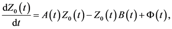
We consider the following boundary value problem
 (1)
(1)
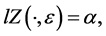 (2)
(2)
where 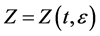 is an unknown operator function from the space
 ,
,  and
and  are bounded operator-valued functions
 ; or in another words these operators are the ways in the space of linear and bounded operators
 ,
,  is a small parameter. We find the solution
  of boundary value problem (1), (2) which for
  turns in one of the solutions
  of the generating boundary value problem
 (3)
(3)
 (4)
(4)
3. A Solvability Criterion and the Structure of the Solution Set of the Nonperturbed Problem
Solutions on the Finite Interval
Consider the case when the differential equation is defined on the finite interval  or on the infinite inter- val. Let us the operator
 ![]() whose action on the operator-valued function
whose action on the operator-valued function ![]() is given by the formula
is given by the formula
![]() (5)
(5)
where![]() ,
, ![]() are evolution operators [13] , of the following operator-differential equations
are evolution operators [13] , of the following operator-differential equations
![]() (6)
(6)
![]() (7)
(7)
respectively. Obviously, that ![]() satisfies the following operator-differential equation
satisfies the following operator-differential equation
![]()
Using the operator![]() , we write out the general solution of the nonperturbed problem
, we write out the general solution of the nonperturbed problem ![]()
![]() (8)
(8)
![]() (9)
(9)
in the form
![]()
where M is an arbitrary operator and
![]()
The main statement of this part is the following theorem.
Theorem 1. Consider the boundary value problem (8), (9).
1) There are exist solutions of the boundary value problem (8), (9) if and only if the following condition is true
![]() (10)
(10)
where![]() , and
, and![]() ; under this condition the family of solutions have the following form
; under this condition the family of solutions have the following form
![]() (11)
(11)
![]()
is generalized Green’s operator and ![]() is Moore-Penrose pseudoinvertible;
is Moore-Penrose pseudoinvertible;
2) There are exist generalized solutions of boundary value problem (8), (9) if and only if
![]()
where ![]() is strong generalized invertible operator. Then the family of solutions of the Equation (8) has the form
is strong generalized invertible operator. Then the family of solutions of the Equation (8) has the form
![]() (12)
(12)
where
![]()
is generalized Green’s operator.
3) There are exist the quasisolutions if and only if ![]() and in this case we have the solutions in the following form
and in this case we have the solutions in the following form
![]() (13)
(13)
with the same generalized invertible.
Sketch of the proof: Substituting in the boundary condition we will have
![]() (14)
(14)
and then we obtain the following operator equation
![]() (15)
(15)
Using the notion of generalized invertible operator [14] [15] , we have the following variants for the equation:
1) If ![]() then Equation (15) has the solution if and only if the following condition is true
then Equation (15) has the solution if and only if the following condition is true
![]() (16)
(16)
If the condition (16) is satisfied then the set of the solutions of the Equation (15) has the following form:
![]()
for any linear and bounded operator C. Then the family of solutions of the boundary value problem (8), (9) has the form
![]() (17)
(17)
where
![]()
is generalized Green’s operator.
2) If![]() . If the
. If the ![]() we have the generalized solutions in the following form
we have the generalized solutions in the following form
![]()
if and only if the following relation is hold
![]()
where ![]() is strong generalized invertible operator [15] . Then the family of solutions of the boundary value problems (8), (9) has the form
is strong generalized invertible operator [15] . Then the family of solutions of the boundary value problems (8), (9) has the form
![]() (18)
(18)
where
![]()
is generalized Green’s operator.
3) If the ![]() we have the quasisolutions in the form
we have the quasisolutions in the form
![]() (19)
(19)
with the same generalized invertible (see also the paper [16] ).
4. Weakly Nonlinear Case
4.1. Necessary Condition
Now we consider the boundary value problem (1), (2). We find the solution ![]() of the boundary value problem (1), (2) which for
of the boundary value problem (1), (2) which for ![]() turns in one of the solutions
turns in one of the solutions ![]() of boundary value problem (8), (9). Now we obtain the necessary condition of the existence of such solutions.
of boundary value problem (8), (9). Now we obtain the necessary condition of the existence of such solutions.
Theorem 2. (necessary condition) Let the boundary value problem (1), (2) has the solution ![]() which for
which for ![]() turns in one of the solution
turns in one of the solution ![]() with operator
with operator![]() . Then the operator
. Then the operator ![]() satisfies the following operator equation for generating operators
satisfies the following operator equation for generating operators
![]() (20)
(20)
Proof. Suppose that the boundary value problem (1), (2) has solution ![]() which for
which for ![]() turns in one of the solutions
turns in one of the solutions ![]() with C0. By virtue of the theorem 1 thefollowing condition of solvability is true
with C0. By virtue of the theorem 1 thefollowing condition of solvability is true
![]() (21)
(21)
where
![]()
Such as condition (10) is true, then the condition of solvability (21) we can rewrite in the following form
![]()
Dividing by ![]() and passing to the limit when
and passing to the limit when ![]() tends to zero we obtain
tends to zero we obtain
![]()
or in the form
![]() (22)
(22)
From this condition we obtain the theorem 2.
4.2. Sufficient Condition of the Solvability
Now we obtain the sufficient condition of the solvability of boundary value problem (8), (9). We make the change of the variable ![]() by the rule
by the rule![]() . Then we obtain the following boundary value problem
. Then we obtain the following boundary value problem
![]() (23)
(23)
![]() (24)
(24)
The family of solutions of the Equation (23) has the following form
![]() (25)
(25)
![]() (26)
(26)
under condition (21)
![]() (27)
(27)
Substituting in this expression (25) and using the Equation (20), we have
![]() (28)
(28)
Then we can rewrite this expression in the following form of the operator equation
![]() (29)
(29)
where
![]() (30)
(30)
and
![]() (31)
(31)
If the following condition
![]() (32)
(32)
is true then the equation (30) has the solution
![]() (33)
(33)
Under condition (32), we can prove that boundary value problem (23), (24) have solutions. In a such way, we prove the following theorem.
Theorem 3. (sufficient condition) Under condition (32) boundary value problem (23), (24) is solvable. Solution of the given boundary problem can be found with using the following converging iterative process
![]() (34)
(34)
![]() (35)
(35)
![]() (36)
(36)
with zero initial data.
Proof.
Proof of this theorem uses the modification of the fixed point theorem and is performed as well as the proof of the theorem 3 from the paper [17] .
Example 1.
Considering the following boundary value problem with the matrix-valued in l2 functions,
![]() (37)
(37)
nonhomogenous part has the following form
![]() (38)
(38)
and conditions on infinity
![]() (39)
(39)
In this case
![]() (40)
(40)
![]() (41)
(41)
Operator ![]() has the following form
has the following form
![]() (42)
(42)
with ![]() *-star matrix which has the following form
*-star matrix which has the following form
![]() (43)
(43)
![]() (44)
(44)
In this case, the operator ![]() has the following form
has the following form
![]() (45)
(45)
From the condition (39) we obtain that![]() ,
, ![]() etc. and
etc. and![]() ,
, ![]() etc. we can take arbitrary.
etc. we can take arbitrary.
In the such way, we have
![]()
(46)
The unperturbed problem has the following form
![]() (47)
(47)
![]() (48)
(48)
Consider the following problem with the matrix,
![]() (49)
(49)
nonhomogenous part has the following form
![]() (50)
(50)
In this case
![]() (51)
(51)
![]()
where
![]() (52)
(52)
![]()
where
![]() (53)
(53)
Here are ![]() and
and ![]() characteristic numbers of the block of the Fibonacci matrix B.
characteristic numbers of the block of the Fibonacci matrix B.