Shape Identification for Stokes-Oseen Problem Based on Domain Derivative Method

Wenjing Yan^*, Jiangyong Hou

School of Mathematics and Statistics, Xi’an Jiaotong University, Xi’an, China.

DOI: 10.4236/jamp.2015.312191                

Abstract

In this paper, we consider the shape identification problem of a body immersed in the incompressible fluid governed by Stokes-Oseen equations. Based on the domain derivative method, we derive the explicit representation of the derivative of solution with respect to the boundary. Then, according to the boundary parametrization technique, we propose a regularized Gauss-Newton algorithm for the shape inverse problem. Finally, numerical examples indicate that the iterative algorithm is feasible and effective for the practical purpose.

Keywords

Inverse Problem, Shape Identification, Stokes-Oseen Equations, Domain Derivative Method

Received 7 November 2015; accepted 26 December 2015; published 29 December 2015

1. Introduction

The purpose of this paper is to determine a shape of the body located in an incompressible viscous Stokes-Oseen flow by applying a formulation of the domain derivative to a numerical simulation.

Shape inverse problem usually consists in reconstructing or recovering the geometry shapes from the mea- sured (observed) data. This kind of problems usually entails very large computational costs: besides numerical approximation of partial differential equations, it requires also a suitable approach for representing and deform- ing efficiently the shape of the underlying geometry. The control variable is the shape of the domain; the object is to recover the unknown boundary from the data which may be given by the designers.

For the domain derivative method, many people are contributed to it. Kress proposed a quasi-Newton method to solve inverse scattering problem in [1] . Hettlich solved the inverse obstacle scattering problem for sound obstacles problem [2] , and discussed a discontinuity in a conductivity from a single boundary measurement [3] . Chapko et al. dealt with the inverse boundary problem for the time-dependent heat equation only in the case of perfectly conducting and insulating inclusions [4] [5] . Serranho presented a hybrid method for inverse scattering for shape and impedance [6] . Harbrecht and Tausch considered the numerical solution of a shape identification problem for the heat equation [7] . Yan et al. recovered the shape of a solid in the incompressible fluid driven by the Stokes flow [8] , and considered the shape optimization problem of a body immersed in the incompressible fluid governed by Navier-Stokes equations coupling with a thermal model in [9] .

The structure of the paper is as follows. In Section 2, we briefly introduce the shape reconstruction problem of the steady Stokes-Oseen equations. In Section 3, we describe the domain perturbation method which is used for the characterization of the deformation of the shapes, and derive the explicit representation of the derivative of solution with respect to the boundary. This will serve as the theoretical foundation of the Newton method for the approximation solution. Section 4 is devoted to the regularized Gauss-Newton scheme applied to the numerical shape identification problem. The performance of the numerical method is discussed and illustrated by numeri- cal examples.

2. Shape Identification Problem

In this paper, we consider the shape identification of an immersed body in the incompressible viscous fluid which is driven by the steady-state Stokes-Oseen equations,

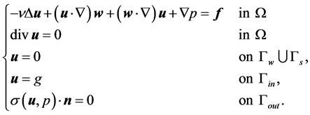(1)

Here denotes the velocity field, is the equilibrium solution of the Navier-Stokes equation, p is the pressure, and is the kinematic viscosity of the incompressible fluid. For a Newtonian fluid the stress tensor is given as with the rate of deformation tensor 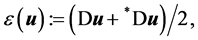where denotes the transpose of the matrix. is the unit normal vector on the smooth boundary which consists of four parts. is the inflow boundary, denotes the outflow boundary, represents the boundary corresponding to the fluid wall, and is the boundary to be recovered. For a given domain, it is well known that this boundary value problem has a unique solution [10] .

The purpose of this paper is to investigate the feasibility of recovering the unknown boundary from the measured (observed) data. We define the operator F on the admissible set X by, where M is the measured (observed) data and may represent a given objective related to specific characteristic features of the incompressible fluid. The inverse problem is both ill-posed and nonlinear.

If and p are smooth functions satisfying (2.1), taking the scalar product of (2.1) with a function we obtain

(2)

where

Throughout the paper we will use the standard notation for Sobolev spaces. Specially, where r is an integer greater than zero, will denote the Sobolev space of real-valued functions with square integrable derivatives of order up to r equipped with the usual norm which we denote. will denote the space of vector-valued functions each of whose n components belong to. We introduce the space

and

3. Domain Derivative Method

In this section, we will discuss how to derive the explicit representation of the derivative of solution with respect to the boundary. This will serve as the theoretical foundation of the numerical algorithm in next section.

A derivative of operator F at boundary can be defined as follows [11] : For any real vector field, we denote the set by

where is small enough. Now we define the domain derivative of F at boundary in the direction by

where the limit should exist uniformly.

Similarly, we denote a perturbation of the interior boundary by

which is a boundary of a perturbed domain, if the vector field is sufficiently small. We

choose an extension of with which vanishes in the exterior of a

neighbourhood of, and define the diffeomorphism in. If the inverse function of is denoted by, and are Jacobian matrices.

Let be the solution of corresponding boundary value problem, i.e. satisfy the variational equation

(3)

for all. Transporting the variables to the reference domain leads to

(4)

for all, where the notations, and.

Denoting the Jacobian of h by. From and, the follow-

ing estimates hold [8]

(5)

(6)

and

(7)

In order to prove the main theoretical result of the paper, we introduce some useful identities (see [2] [12] ) without proof.

Lemma 3.1. If, then the following identity holds:

(8)

where.

Lemma 3.2. Let be a scalar function, and a vector field. The following decom- positions hold:

(9)

(10)

Theorem 3.1. Let, denote the solution of (2.1), and is defined in (3.2). Then is differentiable at in the sense that there exists depending on, such that

(11)

Furthermore, , where the domain derivative satisfies the following equations

(12)

where is the normal component of the vector field.

Proof: Step 1: We establish the continuous dependence of the solution on variations of the boundary. Considering the difference, the variational equation holds

From Equations (3.1) and (3.2), we have

Recall the the approximation (3.3)-(3.5), and set in the last expression

Step 2: In order to show the differentiability, let be the solution of

(13)

for all.

From the properties of forms and, the following expression holds

Considering is the solution of (3.11), we rewrite the above identity as

Let, and employ the norm estimates (3.3)-(3.5) again,

Step 3: We split into and. According to Lemma 2.2, Lemma 2.3 and the divergence for- mula, we obtain

Notice that satisfies the Stokes-Oseen Equation (2.1) and applies the geometrical decompositions formulae, and we can get

From Lemma 3.2, we have the identity,

Considering, the following equation holds

Step (4): Give the conditions on boundaries. It is known that implies. Note that

vanishes on the neighborhood of the boundary,

Thus, satisfies the boundary value problem (3.10). The proof is completed.

4. Numerical Algorithm and Examples

In this section, we will propose a regularized Gauss-Newton algorithm and numerical examples in two dimensions, and the numerical results verify that our methods could be very feasible and effective for the shape inverse problem of the Stokes-Oseen equations.

To our knowledge, there are two groups of approaches for the solution of shape inverse problems of this type, namely regularized Gauss-Newton iterations and decomposition methods. In this paper, we choose the re- gularized Gauss-Newton method. Generally, Newton method is based on the observed information. We define an operator F on set X of admissible boundaries by

(14)

where M is the measured (observation) data [12] , , and is the parametrized form of boundary. However, since the linearized version of (4.1) inherits the ill-posedness, the Newton iterations need to be regularized.

First of all, we apply the following boundary parametrization technique in numerical implementations. Here the parametric representations are denoted by

where is twice differentiable and 2p-periodic with for all. Then, we assume that the orientation of the parametrization is clockwise and the parametrization is counter-clockwise.

(15)

where

with for some fixed number N. Moreover, we set the variation

From the representation (4.2), we have

Now, let for some. We can assign to each

the cost function. In the following, we fix N and Q, and obtain the following theorem as an application of Theorem 3.1.

Theorem 4.1. For the mapping F is differentiable with for and. Here are the solutions to the thermodynamic equations

(16)

where

for.

The numerical algorithm can be organized as follows:

1): Given an initial curve, parametrize it to by the boundary parametrization technique;

2): Solve the direct problem (2.1) by the finite element method;

3): For a given, calculate the discrete domain derivative Equation (4.3) and the Jacobian matrix;

4): Apply the regularized Gauss-Newton method,

where. If

then terminate, where is a regularization parameter; otherwise go back to step (2).

We carry out the numerical examples to demonstrate the feasibility and validity of the proposed algorithm. In the following, we set D to be a rectangle with the fixed boundary, and the boundary of solid S is to be recovered in our simulations. We choose to be different curves:

Case 1: A circle whose center is at the origin with radius 0.6,

Case 2: A cone-shaped curve is denoted by the functions

The dimension of the admissible space is, and the number of observation points is 96. We use the finite element method to solve both the direct and inverse problems. Spatial discretization is effected using the Taylor-Hood pair of finite element spaces on a triangular mesh [13] [14] , that is, the finite element spaces are chosen to be continuous piecewise quadratic polynomials for the velocity and continuous piecewise linear polynomials for the pressure.

For case 1, Figure 1 and Figure 2 give the comparison between the exact curve with the approximate curve for the viscosity coefficient = 0.01 and 0.0025, respectively. For case 2, Figure 3 and Figure 4 display the comparison between the target shape with the reconstructed shape for the viscosity coefficient n = 0.01, 0.005. The numerical examples indicate the feasibility of the proposed algorithm and further research is necessary on efficient implementations.

Figure 1. Case 1: shape reconstruction of a circle, n = 0.01.

Figure 2. Case 1: shape reconstruction of a circle, n = 0.0025.

Figure 3. Case 2. shape reconstruction of a cone-shaped curve, n = 0.01.

Figure 4. Case 2: shape reconstruction of a cone-shaped curve, n = 0.005.

5. Conclusion

This paper is concerned with the numerical simulation for shape identification of the steady Stokes-Oseen problems. The continuous dependence of the solution on variations of the boundary is established, and the repre- sentation of domain derivative of corresponding equations is derived. This allows the investigation of iterative method for the ill-posed problem. By the parametric method, a regularized Gauss-Newton scheme is employed to the shape inverse problem. Numerical experiments indicate the feasibility of the proposed method.

Funding

This work is supported by the National Natural Science Foundation of China (No.11371288).

Conflicts of Interest

The authors declare no conflicts of interest.

References

[1]	Kress, R. and Rundellf, W. (1994) A Quasi-Newton Method in Inverse Obstacle Scattering. Inverse Problems, 10, 1145-1157. http://dx.doi.org/10.1088/0266-5611/10/5/011
[2]	Hettlich, F. (1995) Frechet Derivatives in Inverse Obstacle Scattering. Inverse Problems, 11, 371-382. http://dx.doi.org/10.1088/0266-5611/11/2/007
[3]	Hettlich, F. (1998) The Landweber Iteration Applied to Inverse Conductive Scattering Problems. Inverse Problems, 14, 931-947. http://dx.doi.org/10.1088/0266-5611/14/4/011
[4]	Chapko, R., Kress, R. and Yoon, J.R. (1998) On the Numerical Solution of an Inverse Boundary Value Problem for the Heat Equation. Inverse Problems, 14, 853-867. http://dx.doi.org/10.1088/0266-5611/14/4/006
[5]	Chapko, R., Kress, R. and Yoon, J.R. (1999) An Inverse Boundary Value Problem for the Heat Equation: The Neumann Condition. Inverse Problems, 15, 1033-1046. http://dx.doi.org/10.1088/0266-5611/15/4/313
[6]	Serranho, P. (2006) A Hybrid Method for Inverse Scattering for Shape and Impedance. Inverse Problems, 22, 663-680. http://dx.doi.org/10.1088/0266-5611/22/2/017
[7]	Harbrecht, H. and Tausch, J. (2013) On the Numerical Solution of a Shape Optimization Problem for the Heat Equation. SIAM Journal on Scientific Computing, 35, 104-121. http://dx.doi.org/10.1137/110855703
[8]	Yan, W.J. and Ma, Y.C. (2006) The Application of Domain Derivative for Heat Conduction with Mixed Condition in Shape Reconstruction. Applied Mathematics and Computation, 181, 894-902. http://dx.doi.org/10.1016/j.amc.2006.02.011
[9]	Yan, W.J. and Gao, Z.M. (2014) Shape Optimization in the Navier-Stokes Flow with Thermal Effects. Numerical Methods for Partial Differential Equations, 30, 1700-175. http://dx.doi.org/10.1002/num.21818
[10]	Quarteroni, A. and Valli, A. (1994) Numerical Approximation of Partial Differential Equations. Springer-Verlag, Berlin.
[11]	Pironneau, O. (1984) Optimal Shape Design for Elliptic Systems. Springer, Berlin. http://dx.doi.org/10.1007/978-3-642-87722-3
[12]	Delfour, M.C. and Zolésio, J.P. (2002) Shapes and Geometries: Analysis, Differential Calculus and Optimization, Advance in Design and Control. Springer, Berlin.
[13]	Temam, R. (2001) Navier Stokes Equations, Theory and Numerical Analysis. AMS Chelsea Edition, American Mathematical Society, Rhode Island.
[14]	Gilbarg, D. and Trudinger, N.S. (1983) Elliptic Partial Differential Equations of Second Order. Springer, Berlin. http://dx.doi.org/10.1007/978-3-642-61798-0