The Stability of a Rotating Cartesian Plume in the Presence of Vertical Boundaries ()
1. Introduction
The study of the dynamics of compositional plumes is important for many real life applications in industry ([1] - [6] ), geophysics ([7] -[25] ) and environment ([26] -[34] ). While the presence of the compositional plumes can be harmful (e.g., in iron bars), it is useful in geophysics (e.g., the hot compositional plumes, that rise from the inner core boundary of the Earth into the outer core interact with the rotation and magnetic field of the Earth and may contribute to the Geodynamo). Such a wide range of applications has motivated many studies on various aspects of the dynamics of compositional plumes. These studies are experimental and theoretical. The experimental works on the dynamics of compositional plumes observed that the plume flow seems to be stable (Sample and Hellawell [35] ; Chen and Chen [36] ; Hellawell et al. [37] ). The laboratory studies by Hellawell et al. [37] find that the plumes are thin and long, and its top part tends to break up and disappears. Classen et al. [38] experimentally studied the dynamics of compositional plumes under the influence of vertical rotation to find that the plumes are unstable and break into blobs. On the other hand, the theoretical works on the stability of the plumes showed that the Cartesian plume is always unstable in the absence of rotation (Eltayeb and Loper [16] ) and in the presence of rotation (Eltayeb and Hamza [18] ). These studies assumed that the plume rises vertically in a fluid of unbounded domains. While the experimental studies were conducted in bounded regions to show that the plume was stable, the theoretical models were conducted in unbounded domains to find that the plume was unstable. Thus it is of interest to examine the influence of the vertical boundaries on the dynamics of the plumes. The mathematical model by Al Mashrafi and Eltayeb [6] investigated the influence of the two fixed vertical boundaries on the dynamics of the plumes. They tested the stability of non-rotating Cartesian plumes in a bounded domain to find that the presence of two vertical boundaries affects the stability, but the plumes remain unstable. Moreover, they found that the plume was stable when it was close to the boundary but had a large thickness and the material diffusion is potent in the thin layer between the plume and the nearest boundary.
Motivated by real life applications and laboratory results, we study here the influence of vertical rotation on the dynamics of bounded Cartesian plume. In general, the purpose of this study is to extend the theoretical model by Al Mashrafi and Eltayeb [6] on the dynamics of a Cartesian compositional plume in bounded regions to include the action of vertical rotation. The model by Al Mashrafi and Eltayeb [6] consisted of a column of buoyant fluid of finite thickness,  , rising vertically in another less buoyant fluid bounded by two fixed vertical walls located at
  and
and . The system was infinite in the
  and
and  directions. In the current study, we consider that the whole system rotates about the vertical with a uniform angular speed,
  (see Figure 1).
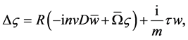
In Section 2, we formulate the model mathematically and state the boundary conditions of the system. The presence of rotation introduces an additional parameter,  , which is a measure of the Coriolis force relative to the viscous force, and this parameter referred to hereinafter as the rotation parameter, defined by
 (1)
(1)
where  is the Taylor number,
  is the kinematic viscosity and
  is the unit of length (see Equation (6) below). In Section 3, we investigate the influence of the vertical boundaries on the linear stability of a rotating

Figure 1. The geometry of the problem showing the profile of the basic state concentration of light material,  , representing a plume of width,
  , and concentration, 1 , rising vertically in a finite fluid of width,
  , and concentration, 0. The system rotates uniformly about the vertical with angular speed,
 . The plume divided the system into three regions: region 2 represents the plume whereas regions 1 and 3 represent the surrounding fluid.
bounded Cartesian plume. The problem of the rotating plume was studied by Eltayeb and Hamza [18] in the absence of boundaries. In Section 4, we discuss the effect of the boundaries on the stability of a rotating plume. The growth rate is maximised over the wave numbers plane  in the parameter space. In Section 5, we make some concluding remarks.
2. Formulation of the Problem
We consider a two-component fluid, in which the concentration of the solvent component (light material) is  and the temperature is
 , rotating uniformly about the vertical with angular velocity
 . The fluid has kinematic viscosity,
  , and thermal diffusivity,
  , and material diffusion is negligible. The dimensionless equations of the system have been derived by Eltayeb and Hamza [18] . They are
 (2)
(2)
 (3)
(3)
 (4)
(4)
 (5)
(5)
Here R,  and
and  are the Grashoff number, the Prandtl number and the rotation parameter, respectively, defined by
 (6)
(6)
where  is the Taylor number and
 ,
,  and
and  are characteristic units of velocity, length and concentration, respectively (Al Mashrafi and Eltayeb [6] ), and
 ,
,  ,
,  ,
,  ,
,  ,
,  ,
,  ,
,  ,
,  are the velocity vector, the pressure, the constant gravitational acceleration, the upward unit vector, the time, the thermal expansion coefficient, the compositional expansion coefficient, the density, the uniform temperature gradient and the subscript “
 ” in the Equation (2) refers to reference values.
We consider a basic concentration profile
 (7)
(7)
which defines a plume of thickness,  , rising with velocity
  in the presence of mean temperature
  and mean pressure
  such that
 (8)
(8)
 (9)
(9)
which are the same equations obtained in the absence of rotation. The presence of rotation does not affect the basic state, and the solution of (8) and (9) is the same as in the absence of rotation. We include it here for easy reference:
 (10)
(10)
where ,
,  and
and  are defined by
 (11)
(11)
3. The Stability Analysis
In this section, we use the perturbation Equations (14)-(17) to investigate the linear stability of the basic state solution given by (10). We assume that the interface at the plane  is given a small harmonic disturbance of the form
 (12)
(12)
where  and
and  are the wavenumber components in the
  plane,
  is the growth rate and
  refers to the complex conjugate.
The disturbance (12) will propagate into the fluid, and affect the second interface and the variables of the system to produce the perturbations. Consequently, the interface at  can be written in the form
 (13)
(13)
where  is a measure of the amplitude of the interface and it is evaluated as a part of the solution. The perturbations introduced into the system are governed by the dimensionless equations (see Al Mashrafi and Eltayeb [6] )

 (14)
(14)
 (15)
(15)

 (16)
(16)
 (17)
(17)
where ,
,  ,
,  and
and  are the perturbations in velocity, pressure, temperature and concentration, respectively.
The perturbation variables take the form
 (18)
(18)
in which the factors ,
,  , and
, and  are introduced in the variables
 ,
,  and
and , respectively, for convenience.
Substituting the variables (18) into the Equations (14)-(17) and after some arrangements we get the following equations
 (19)
(19)
 (20)
(20)
 (21)
(21)
 (22)
(22)
 (23)
(23)
 (24)
(24)
 (25)
(25)
subject to the boundary conditions
 (26)
(26)
 (27)
(27)
 (28)
(28)
 (29)
(29)
where the variable  is related to the vertical component of vorticity and is defined as
 (30)
(30)
and we have introduced the notation
 (31)
(31)
(cf. Al Mashrafi and Eltayeb [6] ).
We use the same method adopted in Al Mashrafi and Eltayeb [6] and expand the perturbation variables and the growth rate in the small parameter , thus
 (32)
(32)
where  indicates any of the perturbation variables
 ,
,  ,
,  ,
,  ,
,  and
and .
.
It turned out that the leading order terms in the equations determines the stability of the system. The relevant equations and the boundary conditions are then obtained from (19)-(24) and (26)-(29) by neglecting the terms with . In order to facilitate comparison with the results of the non-rotating case, we shall maintain the subscript 0. The equations are given by
 (33)
(33)
 (34)
(34)
 (35)
(35)
 (36)
(36)
 (37)
(37)
 (38)
(38)
The associated boundary conditions are obtained from (26)-(29) by introducing the subscript 0 to all the variables and the subscript 1 to .
.
The system (33)-(38) together with the boundary conditions poses an eigenvalue problem for the growth rate,  , which determines the stability of the system. The real part
  governs the variations of the amplitude of the disturbance with time, and hence it determines the stability of the disturbance. If it is negative for all possible values of the wavenumbers
  and
and , then the plume is stable, while if at least one pair of
  and
and  gives a positive value, then the plume is unstable. If
  vanishes for all values of the wavenumbers, the plume is neutrally stable. If the preferred mode occurs for
 ,
,  both non-zero, it is referred to as a 3-dimensional mode (oblique), and if
 , it is called 2-dimensional (vertical). The case
  and
and  is found not to occur. The imaginary part
  determines the phase speed of the disturbance. The vertical phase speed
  and the horizontal phase speed
  are defined as
 (39)
(39)
We note that  is defined only if
 .
.
We operate on Equation (33) with , and use Equations (34)-(36) to get
 (40)
(40)
The general solution of the differential Equation (40) can be written in the form
 (41)
(41)
where the superscript  refers to the three regions of the system (see Figure 1),
  ,
, 
 are constants, and
  are the roots of the cubic equation
 (42)
(42)
with  is given by
 (43)
(43)
We use the Equations (34)-(36) and the solution (41) to obtain
 (44)
(44)
The Equation (37) can be solved in the form a complementary function and particular solution to find
 (45)
(45)
where ,
,  are constants, and
 ,
,  are given by
 (46)
(46)
Now we apply the boundary conditions at ,
,  ,
,  and solve the resulting algebraic equations for the constants
 ,
,  ,
,  ,
,  for
for  The details of the solution are given in the Appendix A.
The growth rate is given by the quadratic equation
 (47)
(47)
where  and
and  are given in the Appendix A.
Solving Equation (47) yields
 (48)
(48)
and the displacement  is given by
 (49)
(49)
in which  and
and  are defined in the Appendix A.
We note that, as in the absence of rotation, the system has two modes. The upper sign in the expression (48) corresponds to the modified varicose mode (MV) and the lower sign refers to the modified sinuous mode (MS).
4. Discussions of the Results
The growth rate (48) is evaluated numerically in the  plane as a function of the parameters
 ,
,  ,
,  and
and  for both modes. The contours of
  in the
  plane are plotted for sample values of the parameters
 ,
,  ,
,  and
and  in the Figures 2-4.
In Figure 2, we present a comparison between the contours of the two modes MV and MS for different values of the Taylor number,  , when
 ,
,  and
and . We note that the MV mode always possesses a minimum with negative growth rate and one or two maxima with positive growth rates while the MS mode has

Figure 2. Contours of the growth rate ,  , of the modes MV, as in (a), (c), (e) and MS, as in (b), (d), (f) for the rotating bounded Cartesian plume where
 ,
,  ,
, . Here
  for (a), (b);
  for (c), (d); and
  for (e), (f). Note that the preferred mode is MS.
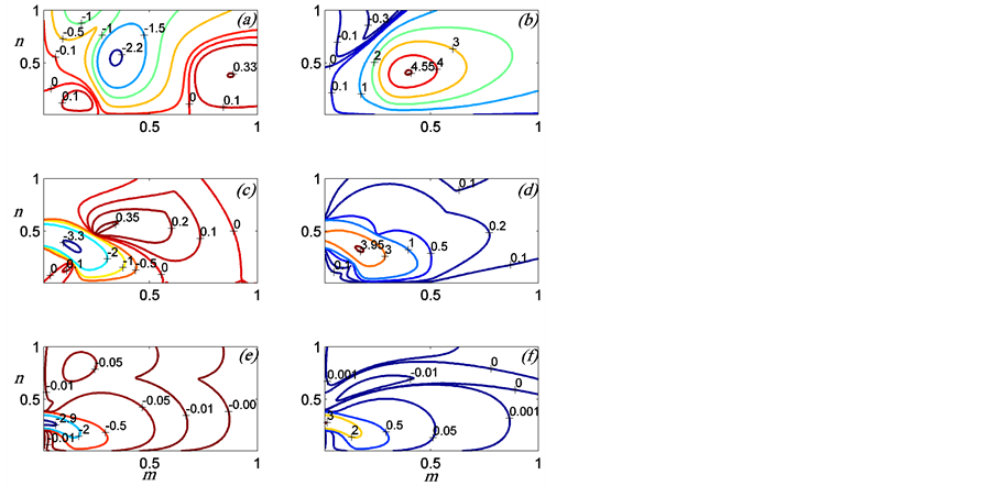
Figure 3. Contours of the growth rate,  , of the modes MV, as in (a), (c), (e) and MS, as in (b), (d), (f) for
 ,
,  ,
, . Here
  for (a), (b);
  for (c), (d); and
  for (e), (f). Note that the preferred mode of the instability is 2-dimensional when
 .
.
a minimum with negative growth rate only when  is small and one maximum with positive growth rate which is larger than that of the corresponding MV mode. This indicates that the MS mode is preferred for this set of parameters. The local maxima correspond to 3-dimensional modes and the largest maximum always increases with the increase in the rotation parameter
 .
.

Figure 4. Isolines of the growth rate ,  , as in (a), (c), (e) and
  as in (b), (d), (f) for
 ,
,  ,
, . Here
  for (a), (b);
  for (c), (d); and
  for (e), (f). Note that at fixed point
 , the values of
  and
and  are nearly same but there different in the sign.
Figure 3 presents the influence of the distance  between the plume and the nearest sidewall on the stability of the plume when the thickness of the plume and the rotation parameter are held fixed at
  and
and . The figure is plotted for three different values of
 :
:  for subfigures (a), (b);
  for subfigures (c), (d); and
  for subfigures (e), (f). When the plume is situated half-way between the sidewalls
 , the MV mode has a negative growth rate everywhere and hence stable while the MS mode has a growth rate that is positive everywhere and hence is preferred. The local maximum possesses a vanishing horizontal wave number and hence propagates vertically. As the plume moves towards a wall, the growth rates of both modes increase and the MV mode develops local maxima with positive growth rates but they are not preferred because the MS mode local maximum increases as well and becomes 3-dimenaional.
Figure 4 illustrates the influence of the plume thickness on the contours of the growth rate for fixed values of the rotation parameter and the distance between the two sidewalls when the plume is situated half-way between the two sidewalls. As  increases from
 , the growth rate for MS mode, which is positive everywhere, increases and that of the MV mode, which is negative everywhere, decreases until
  reaches a critical value,
  , when the growth rate of the MS mode decreases and that of the MV mode increases.
The contours of Figures 2-4 indicate that the preferred mode of instability is the modified sinuous (MS) mode. This indication is quantified by calculating the maximum growth rate and the associated wave numbers and phase speeds for different values of the parameters. For fixed values of ,
,  ,
,  and
and , we maximize over the wave numbers
  and
and  by demanding that
 (50)
(50)
The solution of (50) gives the values  and
and  at maximum growth rate,
  , calculated from (48) for these values of
  and
and  to give, together with the corresponding value
  of the phase speed, the parameters
  of the preferred mode. For fixed parameters
 ,
,  ,
,  and
and , and particular mode, all possible local maxima of
  are identified and the largest value taken together with the corresponding wavenumbers and phase speeds as defining the preferred mode for that set of parameters for that mode. This is carried out for both modified varicose (MV) and modified sinuous (MS) modes, and the largest is chosen as the preferred mode. A sample of the results is given in Figures 5-9.
Figure 5 and Figure 6 illustrate the influence of the distance between the boundaries on the preferred mode of instability of the rotating plume. In Figure 5, the preferred mode parameters are plotted as a function of  for fixed
  and two values of the distance between the sidewalls,
  , for a plume situated half-way between the sidewalls. It is found that the preferred mode is the MS mode and the influence of the boundaries tends to stabilise the plume but only reduces the growth rate slightly. The horizontal and vertical wavenumbers are increased while the phase speeds are reduced as the distance,
  , between the two walls is reduced.
Figure 6 presents the preferred mode of instability as a function of  and fixed
  where the plume is equidistant from the two walls and
  takes the values 10 and 20. The growth rate increases rapidly as
  increases from zero until it reaches a maximum when the plume occupies the middle half of the region between the sidewalls. As the thickness of the plume increases further, the growth rate decreases if
  is small but stays at the maximum value for increasing
  if the distance
  is large. In both case, the growth rate drops to zero as the wall is approached and the plume nearly fill the whole region between the sidewalls. The wavenumbers decrease as
  increases from zero but they soon jump to larger values and increase with
 . In both cases the MS mode is preferred.
Figure 7 illustrates the dependence of the preferred mode on  for
for ,
,  and
and  takes two values:
  and
and . As the Taylor number increases from
 , the maximum growth rate
  increases rapidly until
  reaches a certain value that increases as the distance between plume and the nearest sidewall increases, after which the growth rate varies much more slowly. The wavenumbers of the preferred mode show sudden changes at a small value of
  indicating a change of local maximum as
 , increases through a value,
 . The horizontal wavenumber,
  , is zero for small
  corresponding to 2-dimensional motions, but as
  reaches
 ,
,  jumps to a nonzero value and increases thereafter. The vertical wavenumber increases rapidly as
  increase to
  and then decreases as
  increases further. The vertical phase speed of the preferred mode also suffers a change at
  and the jump depends on how far the plume is from the nearest sidewall.
In Figure 8, we present the dependence of the preferred mode on the distance  between the plume and the nearest sidewall. We note that the growth rate decreases when the plume moves towards the location half-way
between the two sidewalls. Both wavenumber components increase steadily as the distance between plume and the nearest sidewall increases. The vertical phase speed however behaves differently as  increases; it decreases steadily with increasing
  if
if  is small but when
  is large, it decreases slowly reaching a minimum before it increases at a moderate rate. In all cases, it is the MS mode that provides the preferred mode.
Figure 9 shows the dependence of the critical modes  on
on . The growth rate increases gradually until
  reaches a critical thickness,
  , and then it decreases. This indicates that there is a critical thickness representing the most unstable plume. The behaviour of the wavenumber components and phase speed with
  is quite complicated. The horizontal wavenumber vanishes for small
  when
when  is small. For large,
  , behaves in a similar way when
  is close to
 . The vertical wavenumber, on the other hand decreases as
  increases from zero and jumps to a larger value when the local maximum changes, and then varies very slowly until
  is almost 4, when
 .
.
5. Conclusions
The dynamics of a fully developed plume of buoyant fluid, in the form of a channel of finite width,  , rising in a less buoyant fluid contained between two parallel vertical walls, a distance
  apart, and two fluids rotate uniformly about the vertical have been investigated.
In the absence of boundaries ([18] ), it was found that the stability problem depended on the parameters: the Grashoff number,  , the Taylor number,
  , and the thickness of the plume,
 . The magnitude of the growth rate was of the order
  for
for  and the instability took one of the two types: sinuous mode or varicose mode.
The presence of the vertical boundaries here introduces two dimensionless parameters: the distance between the plume and the nearest wall,  , and the distance between the two vertical sidewalls,
 . The introduction of the boundaries modifies the two modes to be the modified sinuous mode (MS) and the modified varicose mode (MV). It is shown here that the boundaries introduce two main effects to the rotating Cartesian plume studied by Eltayeb and Hamza [18] . First, the sidewalls tends to stabilise the plume but succeed only reducing the growth rate and the plume remains unstable for all values of the Taylor number and the distance from the nearest sidewall. Second, the presence of the sidewalls suppresses the modified varicose mode and allows the modified sinuous only to be unstable. The preferred mode can be 3-dimensional or 2-dimensional depending on the values of the parameters of the system. When the preferred mode is 2-dimensional, propagation can be upwards or downwards.
Appendix A: The Derivation of the Dispersion Relation
In this appendix, we apply the boundary conditions (26)-(28) when the subscript is 0 for the variables (41), (44) and (45) to evaluate the constants of the solution. Application of the boundary conditions at the interface  gives
gives
 (A:1)
(A:1)
 (A:2)
(A:2)
 (A:3)
(A:3)
 (A:4)
(A:4)
where ,
,  ,
,  and
and  are defined by
 (A:5)
(A:5)
 (A:6)
(A:6)
 (A:7)
(A:7)
 (A:8)
(A:8)
We use the Equations (A:5)-(A:8) to obtain
 (A:9)
(A:9)
 (A:10)
 (A:11)
 (A:12)
Similarly, at the interface , we find
 (A:13)
 (A:14)
 (A:15)
 (A:16)
in which ,
,  ,
,  and
and  are given by
 (A:17)
 (A:18)
 (A:19)
 (A:20)
Equations (A:17)-(A:20) give
 (A:21)
 (A:22)
 (A:23)
 (A:24)
The boundary conditions at the boundaries  and
and  give
give
 (A:25)
 (A:26)
 (A:27)
 (A:28)
such that ,
,  ,
,  and
and  are defined by
 (A:29)
 (A:30)
 (A:31)
 (A:32)
The equations and can be solved to find
 (A:33)
since the roots  are distinct. Hence Equations (A:3)-(A:5) give
 (A:34)
 (A:35)
 (A:36)
Using the expression for  in , and the properties of the 3 roots of the cubic Equation (42) to simplify the expressions (A:35), (A:36). The simplifications lead to
 (A:37)
Hence the expressions (A:9)-(A:12) reduce to
 (A:38)
 (A:39)
 (A:40)
The same method can be applied to the conditions at . The Equations (A:13)-(A:16) leads to
 (A:41)
thus the expressions (A:21)-(A:24) give
 (A:42)
 (A:43)
 (A:44)
The expressions ,
,  ,
,  and
and , given in (A:29)-(A:32), can be simplified by using the relations (A:38), (A:39) and (A:42), (A:43) to find
 (A:45)
 (A:46)
 (A:47)
 (A:48)
where we have defined the notation
 (A:49)
 (A:50)
 (A:51)
 (A:52)
The Equations (A:49)-(A:52) give
 (A:53)
 (A:54)
 (A:55)
 (A:56)
The boundary conditions at  and
and , given in (A:25) and (A:28), can be written by using (A:45)-(A:48) and (A:55) and (A:56) to obtain
 (A:57)
 (A:58)
in which ,
,  ,
,  ,
,  ,
,  and
and  are defined by
 (A:59)
 (A:60)
and we have defined  and
and ,
,  as
as
 (A:61)
 (A:62)
 (A:63)
 (A:64)
The algebraic system (A:57) and (A:58) can be solved by elimination to find
 (A:65)
in which ,
,  ,
,  and
and  are given by
 (A:66)
 (A:67)
 (A:68)
 (A:69)
 (A:70)
 (A:71)
and we have defined the following notation
 (A:72)
 (A:73)
 (A:74)
 (A:75)
 (A:76)
 (A:77)
 (A:78)
 (A:79)
The constants  and
and  for
for  can easily evaluated using (A:38), (A:39), (A:42), (A:43), (A:53), (A:54). The next step is to find the expressions of the constants
  and
and . The Equations (A:26), (A:27), (A:40) and (A:44) give
 (A:80)
 (A:81)
where  and
and  are defined by
 (A:82)
The application of the boundary condition (29) gives
 (A:83)
such that  and
and  are given by
 (A:84)
where  for
for 
 and
and  are defined by
 (A:85)
 (A:86)
and we have used the notation ,
,  ,
,  ,
,  ,
,  ,
,  and
and 
 (A:87)
 (A:88)
 (A:89)
 (A:90)
 (A:91)
 (A:92)
 (A:93)
and  has the form
 (A:94)
Now the growth rate  and the displacement
  can be evaluated by solving the Equation (A:83) to find
 (A:95)
 (A:96)
where  and
and  are defined by
 (A:97)
 (A:98)