Solution of Differential Equations with the Aid of an Analytic Continuation of Laplace Transform ()
1. Introduction
Yosida [1] [2] discussed the solution of Laplace’s differential equation, which is a linear differential equation, with coefficients which are linear functions of the variable. In recent papers [3] [4] , we discussed the solution of that equation, and fractional differential equation of that type. The differential equations are expressed as
 (1.1)
(1.1)
for  and
and . Here
  for
for  are constants, and
  are the Riemann-Liouville fractional derivatives to be defined in Section 2.
We use ,
,  and
and , to denote the sets of all real numbers, of all integers and of all complex numbers. We also use
 ,
,  ,
,  and
and
 for
for  and
and  satisfying
 . If
. If ,
,  , and
, and
 . We use
  for
for , to denote the least integer that is not less than x. In the present paper, the variable t is always assumed to take values on
 .
.
Yosida [1] [2] studied the Equation (1.1) for  with
with , by using Mikusiński’s operational calculus [5] . In [3] [4] , operational calculus in terms of distribution theory is used, which was developed for the initial-value problem of fractional differential equation with constant coefficients in our preceding papers [6] [7] . In [3] , the derivative is the ordinary Riemann-Liouville fractional derivative, so that the fractional derivative of a function
  exists only when
  is locally integrable on
 , and the integral
  converges.
Practically, we adopt Condition B in [3] , which is Condition 1.  and
and  in (1) are expressed as a linear combination of
  for
for .
.
Here  is defined by
 (1.2)
(1.2)
for , where
  is the gamma function.
We then express  as follows:
 (1.3)
(1.3)
where  are constants, and
  is a set of
 .
.
In a recent review [8] , we discussed the analytic continuations of fractional derivative, where an analytic continuation of Riemann-Liouville fractional derivative of function  is such that the fractional derivative exists when
  is locally integrable on
 , even when the integral
  diverges.
In [4] , we adopted this analytic continuation of Riemann-Liouville fractional derivative, and the following condition, in place of Condition 1.
Condition 2.  and
and  in (1.1) are expressed as a linear combination of
  for
for , where S is a set of
  for some
 .
.
We then express  as follows;
 (1.4)
(1.4)
In [3] [4] , we take up Kummer’s differential equation as an example, which is
 (1.5)
(1.5)
where  are constants. If
 , one of the solutions given in [9] [10] is
 (1.6)
(1.6)
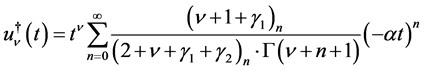
where  for
for  and
and , and
, and . The other solution is
 (1.7)
(1.7)
In [3] , if , we obtain both of the solutions. But when
 , (1.7) does not satisfy Condition 1 and we could not get it in [3] . In [4] , we always obtain both of the solutions. In [1] [2] , Yosida obtained only the solution (1.7).
We now study the solution of a differential equation with the aid of Laplace transform. Then it is required that there exists the Laplace transform of the function  to be determined.
When we consider the Laplace transform of a function  which is locally integrable on
 , we assume the following condition.
Condition 3. There exists some  such that
  as
as .
.
Let  be locally integrable on
  and satisfy Condition 3, and the integral
  converge. We then denote its Laplace transform by
 , so that
 (1.8)
(1.8)
The Laplace transform,  , of
, of  for
for  is then given by
 (1.9)
(1.9)
Let  expressed by (1.3) satisfy Condition 3, and let its Laplace transform
  be given by
 (1.10)
Then we can show that we are able to solve the problems solved in [3] , with the aid of Laplace transform.
When  satisfies Conditions 2 and 3, Laplace transform is not applicable.
In [4] , we adopted an analytic continuation of Riemann-Liouville fractional derivative, by which we could solve the differential equation assuming Condition 2. The analytic continuation is achieved with the aid of Pochhammer’s contour, which is used in the analytic continuation of the beta function.
We now introduce the analytic continuation of Laplace transform with the aid of Hankel’s contour, which is used in the analytic continuation of the gamma function. We then show that (1.9) is valid for , and that if
  expressed by (1.4) satisfies Condition 3, and its analytic continuation of Laplace transform of
 , which we denote by
 , is given by
 (1.11)
then we can solve the problems solved in [4] , with the aid of the analytic continuation of Laplace transform.
In Section 2, we prepare the definition of analytic continuations of Riemann-Liouville fractional derivative and of Laplace transform, and then explain how the equation for the function  and its fractional derivative in (1.1) are converted into the corresponding equation for the analytic continuation of Laplace transform,
  , of
, of , and also how
  is converted back into
 . After these preparations, a recipe is given to be used in solving the fractional differential Equation (1.1) with the aid of the analytic continuation of Laplace transform in Section 3. In this recipe, the solution is obtained only when
  and
and . When
 ,
,  is also required. An explanation of this fact is given in Appendices C and D of [3] . In Section 4, we apply the recipe to (1.1) where
  and
and , of which special one is Kummer’s differential equation. In Section 5, we apply the recipe to the fractional differential equation with
 , assuming
 .
.
In Section 6, comments are given on the relation of the present method with the preceding one developed in [4] , and on the application of the analytic continuation of Laplace transform to the differential equations with constant coefficients.
2. Formulas
Lemma 1. Let  be defined by (1.2). Then for
 ,
,
 (2.1)
(2.1)
Proof. By (1.2), for ,
, . ,
. ,
2.1. Analytic Continuation of Riemann-Liouville Fractional Derivative
Let a function  be locally integrable on
  for
for , and let
  exist. We then define the Riemann-Liouville fractional integral,
  , of order
  by
by
 (2.2)
(2.2)
We then define the Riemann-Liouville fractional derivative,  , of order
 , by
, by
 (2.3)
(2.3)
if it exists, where , and
, and  for
for .
.
For  and
and , we have
 (2.4)
(2.4)
If we assume that  takes a complex value,
  by definition (2.2) is analytic function of
  in the domain
 , and
, and  defined by (2.3) is its analytic continuation to the whole complex plane. If we assume that
  also takes a complex value,
  defined by (2.3) is an analytic function of
  in the domain
 . The analytic continuation as a function of
  was also studied. The argument is concluded that (2.4) should apply for the analytic continuation via Pochhammer’s contour, even in
  except at the points where
 ; see [8] .
We now adopt this analytic continuation of  to represent
 , and hence we accept the following lemma.
Lemma 2. Formula (2.4) holds for every ,
, .
.
By (1.4) and (2.4), we have
 (2.5)
(2.5)
For  defined by (1.4), we note that
  is locally integrable on
 .
.
2.2. Analytic Continuation of Laplace Transform
The gamma function  for
for  satisfying
 , is defined by Euler’s second integral:
 (2.6)
(2.6)
The analytic continuation of  for
for  is given by Hankel’s formula:
 (2.7)
(2.7)
where  is Hankel’s contour shown in Figure 1(a).
We now define an integral transform 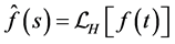 of a function
  which satisfies the following condition.
Condition 4.  is expressed as
  on a neighborhood of
 , for
, for , where
 , and
, and  is analytic on the neighborhood of
 .
.
Let  satisfy Conditions 3 and 4. Then we define
  for
for , by
, by , where
 (2.8)
(2.8)
for , and
, and
 (2.9)
(2.9)
for .
.
Lemma 3. Let  satisfy Condition 4. Then
  defined by (2.8) is an analytic continuation of
 , which is defined by (1.8) for
 , as a function of
 .
.
Proof. The equality  when
when  is proved in the same way as the equality of
  given by (2.6) and by (2.7) for
 ; see e.g. ([11] , Section 12.22). The analyticity of
  and of
  is proved as in ([11] , Sections 5.31, 5.32). Lemma 4. For
 ,
,
 (a)
(a) (b)
(b)
Figure 1. (a) Hankel’s contour CH, and (b) contours CI, −CH and CB which appear in (2.12), (2.15) and (2.16).
 (2.10)
 (2.11)
 (2.12)
where  and
and  are two of the contours shown in Figure 1(b).
Proof. Formula (2.8) for  gives
gives
 (2.13)
for . The last equality in (2.13) is due to (1.9). By using (2.1) and (2.10), the lefthand side of (2.11) is expressed as
 . By replacing
 ,
,  and
and  in (2.13), by
 ,
,  and
and , respectively, we obtain the first equality of (2.12) for
 , with the aid of the formula
 . The equality for
  is obtained by continuity. Theorem 1. Let
  satisfy Conditions 3 and 4 for
 , and
, and  be expressed as
 (2.14)
where  is a finite set of
 . Then the Laplace inversion formula is given by the contour integral:
 (2.15)
where CI is a contour shown in Figure 1(b). Here it is assumed that  is analytic to the right of the vertical line on CI, and is so above and below the upper and lower horizontal lines, respectively, on CI.
Proof. For , the usual Laplace inversion formula applies, so that
 (2.16)
where CB is a contour shown in Figure 1(b). Here it is assumed that  is analytic to the right of the contour CB. By using this with (2.10) and (2.12), we confirm (2.15). Lemma 5. Let
  satisfy Conditions 3 and 4 with an entire function
 . Then
 (2.17)
Lemma 6. Let  be expressed in the form of (1.11). Then the Laplace inversion
  is given by (1.4), provided that the obtained
  satisfies the conditions for
  in Lemma 5, or it is a linear combination of such functions.
Lemma 7. Let  satisfy the conditions for
  in Lemma 5. Then
 (2.18)
 (2.19)
Proof. By using (2.5) and Lemma 4, we obtain these results. ,
3. Recipe of Solving Laplace’s Differential Equation and Fractional Differential Equation of That Type
We now express the differential Equation (1.1) to be solved, as follows:
 (3.1)
(3.1)
where  or
or , and
, and . In Sections 4 and 5, we study this differential equation for
  and this fractional differential equation for
 , respectively.
We now apply the integral transform  to (3.1). By using (2.18) and (2.19), we then obtain
 (3.2)
(3.2)
where
 (3.3)
(3.3)
 (3.4)
(3.4)
Here .
.
Lemma 8. The complementary solution (C-solution) of Equation (3.2) is given by , where C1 is an arbitrary constant and
 (3.5)
(3.5)
where the integral is the indefinite integral and C2 is any constant.
Lemma 9. Let  be the C-solution of (3.2), and
  be the particular solution (P-solution) of (3.2), when the inhomogeneous term is
  for
for . Then
 (3.6)
(3.6)
where C3 is any constant.
Since  in (3.1) satisfies Condition 2 and
  is given by (3.4), the P-solution
  of (3.2) is expressed as a linear combination of
  for
for  for
for , and of
  for
for , respectively.
The solution  of (3.2) is converted to a solution
  of (3.1) for
 , with the aid of Lemma 6.
4. Laplace’s and Kummer’s Differential Equations
We now consider the case of ,
,  ,
,  ,
,  , and
, and . Then (3.1) reduces to
 (4.1)
(4.1)
By (3.3) and (3.4),  ,
,  and
and  are
are
 (4.2)
(4.2)
 (4.3)
(4.3)
4.1. Complementary Solution of (3.2) and (4.1)
In order to obtain the C-solution  of (3.2) by using (3.5), we express
  as follows:
 (4.4)
(4.4)
where
 (4.5)
(4.5)
By using (3.5), we obtain
 (4.6)
(4.6)
in the form of (2.17) or (1.11), where  for
for  and
and  are the binomial coefficients.
If , we obtain a C-solution of (4.1), by using Lemma 6:
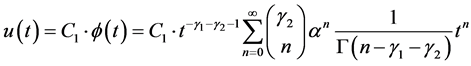 (4.7)
(4.7)
 (4.8)
(4.8)
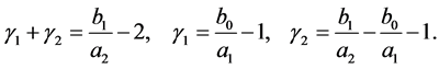
Remark 1. In Introduction, Kummer’s differential equation is given by (1.5). It is equal to (4.1) for ,
,  ,
,  and
and . In this case,
 (4.9)
(4.9)
We then confirm that the expression (4.8) for  agrees with (1.7), which is one of the C-solutions of Kummer’s differential equation given in [9] [10] .
4.2. Particular Solution of (3.2)
We now obtain the P-solution of (3.2), when the inhomogeneous term is equal to  for
for .
.
When the C-solution of (3.2) is , the P-solution of (3.2) is given by (3.6). By using (4.2) and (4.6), the following result is obtained in [3] :
 (4.10)
where
 (4.11)
Lemma 10. When ,
,  defined by (4.11) is expressed as

 (4.12)
where
 (4.13)
This lemma is proved in [3] . In fact, (4.11) is the partial fraction expansion of  given by (4.12) as a function of
 .
.
Applying Lemma 6 to (4.10), and using (4.12), we obtain Theorem 2. Let ,
,  , and let
  for
for . Then we have a P-solution
  of (4.1), given by

 (4.14)
where
 (4.15)
 (4.16)
Here .
.
4.3. Complementary Solution of (4.1)
By (4.3) and (4.5), . When
  and
and , the P-solution of (3.2) is given by
 (4.17)
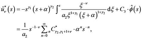
By using (4.14) for , if
, if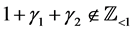 , we obtain a C-solution of (4.1):
 (4.18)
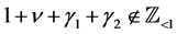
In Section 4.1, we have (4.7), that is another C-solution of (4.1). If we compare (4.7) with (4.15), when , it can be expressed as
 (4.19)
Proposition 1. When , the complementary solution of (4.1) is given by the sum of the righthand sides of (4.8) and of (4.18), which are equal to
  and
and , respectively.
Remark 2. As stated in Remark 1, for Kummer’s differential equation,  and
and  are given in (4.9), and
 (4.20)
We then confirm that if , the set of (4.8) and (4.18) agrees with the set of (1.6) and (1.7).
5. Solution of Fractional Differential Equation (3.1) for 
In this section, we consider the case of ,
,  ,
,  ,
,  ,
,  and
and . Then the Equation (3.1) to be solved is
 (5.1)
(5.1)
Now (3.3) and (3.4) are expressed as
 (5.2)
(5.2)
 (5.3)
(5.3)
5.1. Complementary Solution of (3.2)
By using (5.2),  is expressed as
 (5.4)
(5.4)
where
 (5.5)
(5.5)
By (3.5), the C-solution  of (3.2) is given by
 (5.6)
(5.6)
If , by applying Lemma 6 to this, we obtain the C-solution of (5.1):

 (5.7)
(5.7)
5.2. Particular Solution of (3.2) and (5.1)
By using the expressions of  and
and  given by (5.2) and (5.6) in (3.6), we obtain the P-solution of (3.2), when the inhomogeneous term is
  for
for  satisfying
 :
:
 (5.8)
(5.8)
where  is defined by (4.11) and is given by (4.12).
By applying Lemma 6 to this, we obtain the following theorem.
Theorem 3. Let ,
,  , and let
 . Then we have a P-solution
  of (5.1), given by

 (5.9)
(5.9)
where
 (5.10)
5.3. Complementary Solution of (5.1)
We obtain the solution  only for
 . When
  is given by (5.3) with nonzero values of
 , Theorem 2 does not give a solution of (5.1). Hence
  given by (5.7) is the only C-solution of (5.1).
If we compare (5.7) with (5.10), we obtain the following proposition.
Proposition 2. Let . Then the C-solution of (5.1) is given by
 (5.11)
6. Concluding Remarks
6.1. Solution with the Aid of Distribution Theory
In [4] , the solution of (3.1) is assumed to be expressed as (1.4). In distribution theory, the differential equation for the distribution  is set up, where
  for
for  and
and  for
for . Then it is expressed as
 , where
  is the derivative of order
  in the space of
 of distributions. In [4] , after obtaining
 ,
,  is obtained by using Neumann series expansion. In the present paper,
  is the analytic continuation of Laplace transform of
 . After obtaining
 , we obtain
  for
for  by Laplace inversion.
The steps of solution in [4] and the present paper are closely related with each other, and one may use a favorite one. One difference is that Condition 3 is assumed in the present paper but is not required in [4] .
6.2. Solutions of Differential Equations with Constant Coefficients
We now consider the differential equation given by (3.1), where . Then assuming that the solution
  and the inhomogeneous term
  satisfy Conditions 2 and 3, we show that the analytic continuation of Laplace transform of that equation is given by (3.2) with
 . We then obtain the analytic continuation of Laplace transform of
 ,
, . If it can be expressed as (1.11), then
  is given by its Laplace inverse (1.4). If we take account of Section 6.1, we confirm that the results obtained in [7] are obtained by Laplace inversion.