Travelling Wave Solution of the Fisher-Kolmogorov Equation with Non-Linear Diffusion ()
1. Introduction
For a long time diffusion has been used as a well known model for spatial spread in many biological systems. Okubo [1] and Murray [2] used diffusion in invasion and pattern formation and Skellam [3] studied diffusion in the field of ecology. For motile cell populations diffusion has been used in different situations. Sherrat and Murray [4] used diffusion to model wound healing and Chaplain and Stuart [5] used it to model the capillary growth network.
To study the spatial movement of cell populations, linear diffusion is one of the well known model. However, for closely packed cells such as epithelia, linear diffusion model is unsuitable to examine many biological systems including the movement of cell populations [6]. For closely packed cells, a single cell population can be modeled by a reaction diffusion equation [4,7], but for dissimilar cell populations, a diffusion term would mean that different cell populations can mix together completely and movement of one cells type can be influenced by the cells of other type. But actually the situation is totally opposite, different cell populations cannot move through one another: instead the cell will stop moving when it suddenly comes across another cell. This phenomenon is known as “contact inhibition of migration”. This process has been well documented in many types of cells [8].
In all biological systems the exchange of information at both interand intra-cellular level is almost continuous. In order to get sequential development and generation of the required pattern such communication is necessary e.g. for development and growth of an embryo. Propagating waveforms are one of the ways of conveying such biological information between the cells. Let us consider a simple one-dimensional diffusion equation
 (1)
(1)
where  is chemical (cell or nutrient) concentration and
  is diffusion coefficient. The time to exchange information in the form of changed concentration is
 , where
  is the length of domain. We can get this order by dimensional arguments of Equation (1). At the early stage of growth of an organism the diffusion coefficient can be very small: values of order 10−9 to 10−11 cm2∙sec−1. If diffusion is the main process to convey the biological information then to cover macroscopic distances of several millimeters requires a very long time. When the diffusion coefficient is O (10−9 to 10−11 cm2∙sec−1) and
  is order of 1 mm then the time required to convey the information is O (107 to 109 sec), which is very large in the early stages of growth of an organism. This means that simple diffusion is unlikely to be the main means of exchanging the information during embryogenesis. Karevia [9] and Tilman and Karevia [10] estimated the diffusion coefficient for insect dispersal in interacting population.
About seventy years ago Fisher [11] and Kolmogorov et al. [12] introduced a classical model to describe the propagation of an advantageous gene in a one-dimensional habitat. The equation describing the phenomenon is a one-dimensional non-linear reaction-diffusion equation,
 (2)
(2)
where  is chemical concentration,
  is the diffusion coefficient and the positive constant
  represents the growth rate of the chemical reaction. Since then a great deal of work has been carried out to extend their model to take into account the other biological, chemical and physical factors. The Equation (2) is also used in flame propagation [13], nuclear reactor theory [14], autocatalytic chemical reactions [15,16], logistic growth models [17] and neurophysiology [18].
One of the extensions of the Fisher and Kolmogorov model is to introduce a non-linear diffusion coefficient, which can be taken as a non-linear Fick’s law. The nonlinearity can arise in terms of space, time or density-dependent diffusion coefficient. In the Fisher and Kolmogorov model the reaction kinetics are coupled to diffusion which gives travelling waves of chemical concentration and it can affect biological change very much faster as compared to the processes governed by simple diffusion without the kinetic term. In many biological populations density-dependent dispersal has been observed e.g. Carl [19] observed that ground squirrels move from highly populated area to sparsely populated areas, Myers and Krebs [20] studied the population density cycles in small rodents. Several mathematical models have been developed to describe the density-dependent dispersal systems. Gurney and Nisbet [21,22] developed a first density-dependent diffusion model in ecological context by using a random walk approach and Montroll and West [23] developed a one-dimensional model for a single species by using the same approach. But there is not much work on the Fisher equation with non-linear diffusion. Sánchez and Maini [24] studied a travelling wave solution in a degenerate Fisher equation with non-linear diffusion.
Although Equation (2) is known as the Fisher-Kolmogorov equation, the discovery, investigation and analysis of travelling waves in chemical reactions was first reported by Luther [25]. He found that the wave speed is a simple consequence of the differential equations. He obtained the wave speed in terms of parameters associated with the reactions he was studying. The analytical form is the same as that found by Kolmogorov [12] and Fisher [11].
Seeking the travelling wave solution of Fisher equation has been a challenging and difficult task. Several authors used different methods to find the travelling wave solution of Fisher equation. Ablowitz and Zeppetella [26] obtained the first explicit form of travelling wave solution of Fisher equation using Painlevé analysis. The authors found that kink wave propagates from left to right with a speed . Wazwaz [27] used tanh method to find the travelling wave solution of non-linear partial differential equation. The author also extended this study to the equations which do not have tanh polynomials. He also demonstrated the efficiency of the method by applying it to variety of equations e.g. Fisher equation. Mansour [28] found a travelling wave solution of class of degenerate reaction diffusion equations in which non-linearity is assumed to be singular at zero. He employed two methods to find the wave profile and speed of the front. These method include travelling wave equation and initial boundary value problem with an adaptive travelling wave condition for partial differential equation. Tan et al. [29] used an analytical method namely Homotopy analysis method to solve the Fisher equation and they described a family of travelling wave solutions. Jiaqi et al. [30] found a travelling wave solution of non-linear reaction diffusion equation by using the homotopic method and theory of travelling wave transform. Feng et al. [31] found the travelling wave solution of reaction diffusion equation by two methods. Firstly they applied Divisor theorem for two variables in complex domain to find a quasi-polynomial first integral of an explicit form to an equivalent autonomous system. Then through this first integral, they reduced the reaction-diffusion equation to a first-order integrable ordinary differential equation, and found a class of traveling wave solutions. They compared their results with the existing results and found some errors in analytic results in literature. They clarified and introduced the refined results. Hou et al. [32] studied the travelling wave solution of reaction diffusion equation with double degenerate nonlinearities. They investigated existence, uniqueness and stability of wave solution.
In this paper we study the growth of cells in one-dimensional scaffold in the presence of constant nutrients. We model a system in which cell growth and diffusion takes place simultaneously but the cell diffusion depends on cell density. It increases with increase in cell density. The equation governing this system is a non-linear Fisher equation in which the diffusion coefficient depends on cell density. The non-linearity arises in the diffusion coefficient. We represent the diffusion coefficient as an exponential function of cell density. The form of nonlinear diffusion captures the feature that it is very small for small cell density and increases with the increase in cell density and it is maximum when cells stop growing. Results are presented for different values of the parameters. The Fisher equation has such wide applicability in itself but also it is the prototype equation which admits travelling wavefront solutions. We study the travelling wave solution of this equation and find the approximation for the minimum wave speed. We find that the minimum wave speed depends on the model parameters. For moderately non-linear systems the analytical method correctly predicts the wave speed in our numerical calculations. However for strongly non-linear diffusion the numerical wave speed becomes larger than the analytic minimum speed.
The paper is organized as follows in Sections 2 and 3 we present the dimensional and nondimensional model equations respectively. The parameter values and travelling wave solution are described in Sections 4 and 5, respectively. We present the numerical solution in Section 6 and calculate the numerical minimum wave speed in Section 7.
2. Mathematical Model
In this Section we model cell growth in a bioreactor subject to uniform nutrient concentration. Consider the cells are seeded onto a porous scaffold with interconnected pores, which is placed in the bioreactor. The scaffold extends from , where
  denotes the spatial coordinate. In this model we represent the cell density by
 , initial cell density by
 , maximum carrying capacity of the system by
  and diffusion coefficient by
 . We assume that the environment is inhomogeneous i.e. the cell density
  and diffusion coefficient
  depends on spatial coordinate
  and time
 , i.e.
  and
and . We know that the cells require some nutrients such as oxygen and glucose etc. to live and perform specific functions. Suppose that the concentration of such nutrients remains uniform everywhere in the entire domain at all times. We want to model a system in which the change in cell density is due to cell proliferation and cells disperse in the entire domain due to diffusion. We assume that when the cell density is small diffusion is also very small and when the cell density
  reaches its maximum carrying capacity
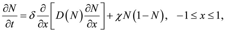
  the cell proliferation stops and cells spread in the entire domain via diffusion. For that we consider a logistic growth model in which the cell population spreads via diffusion. That means we have a coupled system of reaction kinetics and diffusion. Our modelling of cell proliferation [33,34] has led us to the following Fisher equation with non-linear diffusion.
 (3)
(3)
where  is the maximum cell growth rate and
  is the non-linear diffusion. We observe that cells grow in numbers due to second term on the right hand side of Equation (3) and they disperse in the entire domain due to first term on the right hand side of Equation (3). To model cell proliferation we need to choose a form of
  so that, in regions of low cell density, cells grow by increasing their density with little or no spatial motion, whereas in regions of high cell density the newly formed cells diffuse rapidly towards regions of lower cell density. Thus to model this behaviour on a continuum level we choose the following form for the non-linear diffusion.
 (4)
(4)
where parameter  is the cell diffusion when cell density
  reaches its maximum carrying capacity
 , so we can call this the maximum value of cell diffusion and the parameter
  controls how fast cells are spreading in the domain. The parameters
  and
and  have dimensions m2/sec and m3/cell respectively. The exponential function in Equation (4) ensures that cell diffusion will remain positive. The non-linear cell diffusion
  also has maximum value
  when
when . So we can say that non-linear cell diffusion is maximum either when cell density
  reaches its maximum carrying capacity
  or the value of parameter
  is zero. The non-linear diffusion becomes linear when
 . It is also clear from the Equation (4) that when there are no cells then in that case cell diffusion is
 , which is the minimum value of diffusion. So cell diffusion varies in the range,
 (5)
(5)
Initially when the cell density  is small, the diffusion coefficient
  is also small and
  increases with increasing cell density
  but it always remains positive.
The initial cell density  is given by
 (6)
(6)
3. Nondimensionalization
For convenience and to reduce the parameters in the equation we rescale all the variables to analyze the nondimensional form of the equation. We nondimensionalize all lengths by  which we take as a typical length scale for the problem and all cell densities by the maximum carrying capacity
 .
.
 (7)
(7)
 (8)
(8)
We nondimensionalize time by the speed of the growth front  (which is given by Equation (30)),
 (9)
(9)
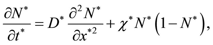
In dimensionless form Equation (3) can be written as
 (10)
(10)
where 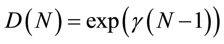 and
and . The parameters
  and
and  are dimensionless parameters in the model which are given by
 (11)
(11)
The parameter  is the ratio of cell growth rate to speed of growth front and parameter
  is the ratio of maximum value of non-linear diffusion to the speed of growth front. The parameter
  controls the diffusion and the parameter
  controls the growth term. The initial condition (6) in dimensionless form becomes
 (12)
(12)
4. Parameter Values
The modified Fisher Equation (10) includes a number of parameters. Some parameters depend on the cell type and some parameters depend on scaffold geometry. Table 1 shows the values of the parameters used in the simulation. We assume that the length  of the scaffold is 0.02 m. Some quantities such as cell growth rate depend on the cell type cultured in the bioreactor. The above proposed model is a generic model and can be applied to any cell type. To compare the model with the experimental data the cells used in the simulations are Murine immortalized rat cell
 . The maximum cell growth rate
  for
for  cells is
  [35]. Since cell growth is a slow process we can choose that speed of growth front
 is very small e.g.
 . The value of dimensionless parameter
  can be obtained by using the values of dimensional parameters
 ,
,  and
and . The values of parameters
  and
and  are not available in the literature. To estimate the value of these parameters we use the expression for dimensionless wave speed i.e.
 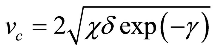 (which we will calculate later in Section 5.2). We choose that the theoretical wave speed
 . In the expression for
  there are two unknowns
  and
and . In order to find the value of
  and
and  we fix one of the parameters
  or
or  in the expression for
 . If we fix the parameter
  then using the expression for
  we can find the value of parameter
 . We observe that the value of dimensionless parameter
  depends on the value of parameter
 . If the value of parameter
  is high then value of
  is also high. This means that cells will diffuse more quickly for high values of parameter
 . Table 1 shows the values of the dimensional parameters used in the model. We know that the initial cell density
 . We can use any form of
 .
.
5. Travelling Wave Solution
We are interested in travelling wave solutions because Equation (10) has two steady states  and
and , which are, respectively, unstable and stable. This suggests that we should look for a travelling wave solution of Equation (10) for which
 ; since negative cell density has no physical meaning. If a travelling wave solution exists it can be written in the form
 (13)
(13)
where  is the wave speed. Since Equation (10) is invariant if
 ,
,  may be negative or positive. To be specific we assume that
 . We have
 (14)
(14)
Substituting the travelling wave solution (13) into Equation (10) and using relations from Equation (14) we get a second order ordinary differential equation,

Table 1. Model parameters used in this work.
 (15)
(15)
where
 (16)
(16)
where primes denote the differentiation with respect to . A typical wave front solution is a solution such that
  approaches one steady state as
  and approaches the other steady state as
 . Therefore the boundary conditions for travelling wave solution are
 (17)
(17)
5.1. Phase Plane Analysis
From Equation (15) we observe that we have to determine the values of the wave speed  such that a nonnegative solution
  of Equation (15) exists. We use phase plane analysis to characterize solutions of Equation (15) in the
  phase plane where,
 (18a)
(18a)
 (18b)
(18b)
The system of ordinary differential Equations (18) is nearly singular at , since
  for high values of parameter
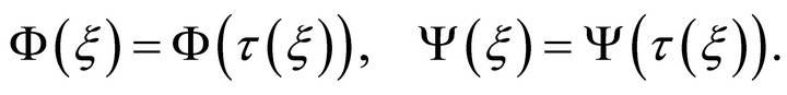
 . To remove the near singularity we introduce a new parameter [24],
  in such a way that
 (19)
(19)
Except at , where
  is not defined,
 .
.
Thus we have
 (20)
(20)
and we obtain
 (21)
(21)
Substituting  and
and  into the system of Equations (18) we get
 (22a)
(22a)
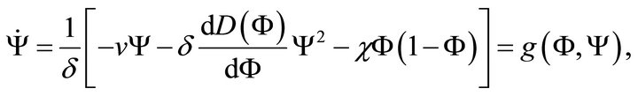 (22b)
(22b)
where dot denotes the derivative with respect to .
.
The phase trajectories of (22) are solutions of
 (23)
(23)
The fixed points  are the points where
 , these are steady states. So in this case fixed points are
  and
and . The local behaviour of the trajectories of system (22) can be obtained by analyzing the linear approximation of system (22) around each fixed point.
5.2. Stability of Fixed Points
The system of Equations (22) has two fixed points, but which of these fixed points are stable? The local stability of a fixed point  is determined by linearization of the dynamics at the intersection. So with the linear approximations the system of Equation (22) becomes
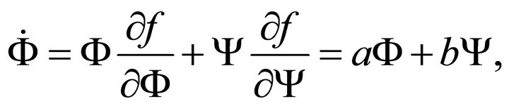 (24a)
(24a)
 (24b)
(24b)
which can be written in the matrix form as
 (25)
(25)
where
 (26)
(26)
Let  and
and  be eigenvalues of
  then we have


 (27)
(27)
where
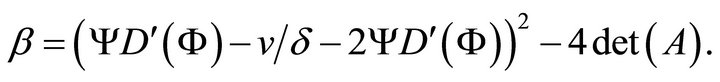
Eigenvalues  for the fixed points (0, 0) and (1, 0) are
 (28a)
(28a)
 (28b)
(28b)
We know that  and
and . Using values of
  and
and  in Equation (28) we get
 (29a)
(29a)
 (29b)
(29b)
It is clear from the Equation (29a) that fixed point  is a stable node if
 , with the case when
  giving a degenerate node. The fixed point (0, 0) is a stable spiral if
  or
or ;
;
i.e.  oscillates in the vicinity of origin. When
 then it is not physically realistic because
  cannot be negative. The fixed point
  is a saddle point. The solution of our modified Fisher equation evolve to a travelling wave if the fixed point
  is a stable node and minimum wave speed of wave front is
 . The condition that
  is a stable node is a necessary condition for travelling wave propagation but not sufficient. Sometimes it gives wrong answer as we shall in see Section 7. If the propagation speed of the front is determined by the leading edge of the population distribution the non-linear fronts whose asymptotic propagation speed equals
  is called a “pulled front”. In this case the eigenvalues give the right answer because the wave speed is determined by what happens at the front edge where
 . As above
  is determined by the eigenvalues thus we call
  speed of pulled front. On the other hand if the speed of front is determined by the whole wave-front but not the behaviour of the leading edge the front is called the “Pushed front” [36,37]. In this case simply computing the eigenvalues gives the wrong answer for the minimum wave speed and the minimum wave speed is
 .
.
Thus the wave speed for a pulled front is given by
 . The wave speed
  depends on the parameters
 ,
,  and
and , is directly proportional to the square root of the product of
  and
and . In terms of the original dimensional Equation (3) the wave speed
  is
is
 (30)
(30)
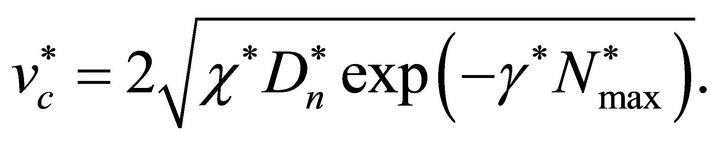
We observe from the system of equations (28) that for a general function  the wave speed
  is determined by
 . So in general the wave speed of the Pulled front is
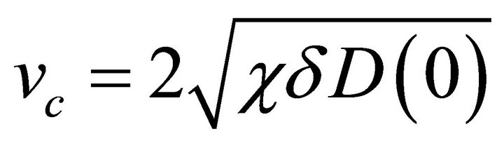 .
.
Figure 1 shows the phase plane sketch of the trajectories of Equation (22) when . We see that when

Figure 1. Phase plane trajectories of Equation (22). Here parameter values are χ = 132.1739, δ = 0.0139 γ = 2 and v = 1.5 > vc. For explanation of parameter values see Section 4.
 the fixed point
  is a stable node because all the trajectories from
  to
to  have the same limiting direction towards
  and the fixed point point
  is a saddle point because there are two incoming trajectories and two out going trajectories and all the other trajectories in the neighborhood of the critical point
  bypass
 . Similarly Figure 2 shows the phase plane sketch of the trajectories of Equation (22) when
 . We observe that when
  the fixed point
  is a stable spiral because all the trajectories from
  to
to  spiral around the point
 .
.
Figures 3 and 4 show the phase plane sketch of trajectories of Equation (22) for various wave speeds  and
and  respectively. We observe from the Figure 3 that when
  all the trajectories in the phase plane
  from
from  to
to  remain entirely in the quadrant where
  and
and , with
  for all wave speeds
 . Similarly from the Figure 4 we see that for all wave speeds
  the phase trajectories from
  to
to  spiral around the fixed point
 . In this case
  oscillates in the vicinity of the origin giving
  negative which is unphysical.

Figure 2. Phase plane trajectories of Equation (22). Here parameter values are χ = 132.1739, δ = 0.0139, γ = 2 and v = 0.5 < vc. For explanation of parameter values see Section 4.

Figure 3. Phase plane trajectories of Equation (22) for different values of v ≥ vc. The other parameter values are same as in Figure 1. Each curve (starting from bottom) represents the trajectory for various values of speed v ≥ vc, i.e. v = 1, v = 1.5, v = 2, v = 2.5 and v = 3 respectively.

Figure 4. Phase plane trajectories of Equation (5.1) for different values of v < vc. The other parameter values are same as in Figure 1. Each curve (starting from bottom) represents the trajectory for various values of speed v < vc, i.e. v = 0.5, v = 0.6, v = 0.7 and v = 0.8 respectively.
5.3. Selection of Initial Condition
A very important question at this stage is what kind of initial condition  will evolve into the travelling wave solution and if the travelling wave solution exists what is its wave speed
 ? Fisher [11] found that Equation (10) has an infinite number of travelling wave solutions for which
  for all wave speeds
 . Kolmogorov [12] proved that Equation (10) has a travelling wavefront solution and the wave speed is
 , if
, if  has compact support. A function
  is said to have a compact support if
 (31)
(31)
where

where  and
and  is continuous in
 . If the initial condition is other than (36) then solution depends on the behaviour of
 .
.
If  then Equation (15) reduces to
 (32)
(32)
A travelling wave solution of Equation (32) in explicit form for  was found by Ablowitz and Zeppetella [26] for the special wave speed
 ,
,
 (33)
(33)
But if  is not a constant then it is not possible to find the exact solution of Equation (15). Solution of such non-linear problem can be approximated by perturbation theory or numerical investigation.
6. Numerical Solution
Numerically we solve the modified Fisher Equation (10) by using the commercial finite element solver COMSOL. We subdivide the domain  into a suitable number of mesh elements (intervals) of length
 . The end points of each interval are called node points and the elements do not have to have the same length. But in this case the length
  of each element is same. To obtain meaningful results care is required in the choice of a suitable number of mesh elements, finite element approximation and model parameters. Convergence is achieved by successively refining the mesh elements. The refined mesh contains 30,721 mesh vertices and 30,720 mesh elements. The dependent variable
  is approximated by a quadratic shape function and solved for 61,441 degrees of freedom. We assume that at time
  the cell density is
  and after the time
  the cell density is
 . We start with initial cell density
  and after each time
  we replace
  by
by  and solve the Equation (10) again for updated cell density. The time from
  to
to  is subdivided as
 , where
  is the time step size from
  to
to  and
and  is the time when we update the cell density. The cell density
  at each mesh point
  is obtained for different times. To estimate the wave speed
  numerically we look for the point
  after each time
  where the cell density is half of its maximum value i.e.
 . When the cell density is half of its maximum value at time
 , then
  and at time
 ,
, . So we can estimate the total distance
  traveled by the wave in the time interval
 . Hence
 (34)
(34)
Results are plotted for different values of the dimensionless parameters  and
and  in Sections 6.1 to 6.4. In the next Section we consider various cases in which we fix the value of dimensionless parameter χ and vary the values of dimensionless parameter
  and parameter
  in such a way that the theoretical wave speed
remains 1. Let us assume that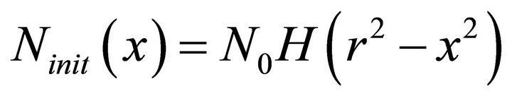 where N0 and r are constants and
  is the Heaviside step function.
6.1. Case I: χ = 1.3217
In this case we fix the value of dimensionless parameter  and find the values of parameter
  and
and  such that theoretical speed of growth front
  is 1. Table 2 shows the values of dimensionless parameter
  for corresponding values of parameter
 .
.
Figures 5 and 6 show the numerical solution of the modified Fisher Equation (10) for the parameter values given in the Table 2. We observe from Figures 5 and 6 that the solution does not evolve into a travelling wave solution before it reaches the domain edges. The cell density  drops down because the rate of diffusion is larger than the growth rate, which means that the dimensionless parameter
  is larger than the dimensionless parameter
 . Diffusion dominates in this simulation so we need to look at the case where diffusion is smaller and cell growth is larger, to find a travelling wave. Numerical results are plotted for
  and
and  in Figures 5 and 6. In a larger domain and with a longer time of solution the system will eventually evolve into a travelling wave but we are interested in a finite domain.
6.2. Case II: χ = 13.2173
We consider the case when the dimensionless parameter

Figure 6. Numerical results of profile of cell density N at different times when γ = 2, δ = 1.3976, χ = 1.3217. Ninit, Δt and tnew are same as in Figure 5.
 and find the value of parameter
  and
and  such that theoretical speed of growth front
  is 1. Table 3 shows the values of dimensionless parameter
  for the corresponding values of parameter
 .
.
Numerical results of modified Fisher Equation (10) are plotted in Figures 7 and 8 for parameter values given in Table 3. It is clear from the Figures 7 and 8 that in this case the solution evolves into travelling wave fronts. So in this case the growth term is somewhat larger than the diffusion term. But the diffusion term is not too small because the cells also diffuse very quickly. This feature is evident from the Figures 7 and 8 because at the edges the front are smooth.
6.3. Case III: χ = 132.1739
Consider the case when the value of dimensionless parameter  is very high i.e.
  and we find the values of parameters
  and
and  such that theoretical speed of growth front
  is 1. Table 4 shows the values of dimensionless parameter
  for corresponding values of parameter
 .
.
In the modified Fisher Equation (10), growth and diffusion are taking place simultaneously. But if the diffusion is very small compared to growth, then first cells will grow quickly and when they reach maximum carrying capacity growth stops and they spread in the domain via diffusion. In the present case the growth term is very big as compared to the diffusion term.
Figures 9 and 10 show the numerical solution of the modified Fisher’s Equation (10) for  and values of parameters
  and
and  given in Table 4. The wave front takes some time to settle down to a travelling wave, which moves at a constant speed. When the number of cells reaches its maximum limit the proliferation
stops and then the cells spread via diffusion in the entire domain. In this case diffusion term is much smaller than the growth term, and due to this reason the shape of the front is very sharp. It is evident from the Figure 9 and 10 that when the front settles down then it moves with
constant speed and shape.
6.4. Case IV: χ = 0
If  then it represents the case when there is no growth of cells. The number of cells will not increase because of the absence of growth term. In that case for every value of
  the solution will not evolve into a travelling wave. Figures 11 and 12 show the cell density in the pure diffusion case i.e. Fisher equation without the growth term for the same times and parameter values used in Figure 7 except in this case
 . The behaviour of the solution is different from the Fisher equation

Figure 11. Numerical results of profile of cell density N at different time without growth term when γ = 1, δ = 0.05141, χ = 0. Ninit, Δt and tnew are same as in Figure 5.

Figure 12. Numerical results of profile of cell density  at different time without growth term when γ = 2, δ = 0.139760, χ = 0. Ninit, Δt and tnew are same as in Figure 5.
with the growth term. Clearly the solution does not grow due to the absence of growth term and the behaviour of the solution is not wave-like.
7. Numerical Minimum Wave Speed
From the phase plane analysis it is clear that a travelling wave front solution exists for a range of wave speeds . We choose the values of parameters
  and
and  such that the theoretically wave speed
 . If diffusion is linear in the modified Fisher Equation (10) then travelling wave move with the minimum wave speed
  [2]. In this model
  corresponds to linear diffusion. But when the value of
  then diffusion is no longer linear. Here we see that the numerical wave speed agrees with the theoretical value when
 . However at
  the numerical speed begins to diverge from the theoretical value and become increasingly large as
  increases.
Figures 13 and 14 show the phase plane sketch of the trajectories of Equation (10) for  and
and  respectively. We observe from the Table 5 that when
  and
and  the numerical value of the minimum wave speed
 . We see that from Figure 13 that when
  then all trajectories from
  to
to  remain entirely in the region where
  and
and  for all wave speed
 . Similarly from Figure 14 we observe that when wave speed
  then for all the trajectories from
  to
to ,
,  becomes negative, which is unphysical.
  is still a stable node. We observe that method of finding
  by looking at the eigenvalues gives the wrong answer. It is beyond the scope of this work to find the analytical formula for the minimum wave speed
 , because the solution depends on the whole trajectory, but we have a very good agreement between numerical results and phase plane analysis.

Figure 13. Phase plane trajectories of Equation (24) for different values of . The other parameter values are χ = 132.1739, γ = 3, and δ = 0.037990. Each curve (starting from bottom) represents the trajectory for various values of velocity
  i.e. v = 1.15, v = 1.2, v = 1.3 and v = 1.5.

Figure 14. Phase plane trajectories of Equation (24) for different values of . The other parameter values areχ = 132.1739, γ = 3, and δ = 0.037990. Each curve (starting from bottom) represents the trajectory for various values of velocity
  i.e. v = 1, v = 1.02, v = 1.05 and v = 1.09.

Table 5. Numerical minimum wave speed .
.
Figure 15 shows the shape of growth front at time  for fixed value of
  but different values of
  and
and . It is evident from Figure 15 that the speed of the growth front is not the same for all values of parameter
 . The speed of the growth front depends on the value of
  and increases as value of
  increases.