VaR-Optimal Risk Management in Regime-Switching Jump-Diffusion Models ()
1. Introduction
In this paper we study a classical hedging policy based on options followed by an institutional manager whose aim is to minimize the Value-at-Risk of a position in a regime-switching jump-diffusion market. Although sharply criticized for the lack of sub-additivity and its inability to quantify the severity of an exposure to rare events, VaR has been adopted as a benchmark in the financial industry and for regulatory purposes. It plays a central role in banking regulation and internal risk management, mainly due to its simplicity. The analysis of this hedging strategy has been initiated by [1] a decade ago for a portfolio made by a risky asset following a lognormal random dynamic, and hence analytically solved in a Black-Scholes setting. More recently, it has been considered for a bond portfolio in [2,3]. By taking the VaR as the risk measure for potential losses L of a portfolio, we hedge the risky position by buying a fraction h of a put option with maturity T and strike price K: but what K and h? By fixing a hedging constraint, the corresponding (constrained) optimality condition involves quantiles computations and derivative pricing. Both steps can be efficiently faced with the Fourier transform technique, under historical and risk-neutral probability respectively.
The dynamic model we consider for the risky position is , where
  is specified on a filtered probability space as a jump-diffusion whose parameters change over time, driven by a continuous time and stationary Markov Chain on a finite state space
 , representing the unobserved state of the world. In fact, empirical studies on the behavior of financial markets show the ability of regime-switching models to capture some peculiarities in the observed data, as firstly highlighted in the seminal paper by Hamilton [4]. Since then, there has been a growing effort in applying switching models to a wide class of financial and/or economic problems. On the other hand, the necessity of including jumps in the underlying models to provide better representation of their dynamical properties is widely recognized (see e.g. [5]). Empirical stylized facts about observed data, such as volatility clustering and heavy tails, are then well captured by regime-switching jumpdiffusions which turns out to be an appealing and flexible class of dynamic models. The computation of quantiles in regime-switching models has been considered by several authors mainly in discrete-time setting (see e.g. [6,7] and ref. therein). Here we consider this problem in the continuous time framework in which the required computations can be very efficiently implemented with the help of Fourier Transform methods (see e.g. [8]). The use of this kind of technique for the analytical calculation of VaR has been considered in Duffie and Pan [9] in terms of the Fourier inversion of the characteristic function. The use of Generalized Fourier Transform and the FFT algorithm is more recent: see Le Courtois and Walter [10], Kim et al. [11] and Scherer et al. [12].
The paper is organized as follows: we firstly derive the optimality conditions for the VaR minimizing strategy (Section 2) and then (Section 3) we introduce the regimeswitching dynamic model, its generalized characteristic function and the change-of-measure result for switching from the historical to the risk-neutral probability. Finally, in Section 4 we specify the Fourier Transform technique for calculating quantiles and put/call option prices and report some numerical experiments to show the impact of jumps and regime-switching on the optimal hedging strategy.
Some final comments can be briefly outlined. Firstly, the analysis of the hedging strategy is fairly general, that is it can be applied to any dynamical model for which Fourier transform methods are viable, for example it can be extended to Variance-Gamma or Bates models. Furthermore, besides the choice of different dynamic models, it would be interesting to consider alternative risk measures, such as the Conditional Value at Risk (CVaR). This is certainly less commonly used in finance industry, but it is widely used in insurance industry being a coherent, convex and stable risk measure (see [13]).
2. VaR and Optimal Risk Management
Given a confidence level , the set of
  -quantiles of the random variable
  is the interval
 where
where
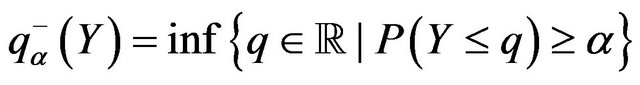 and
and
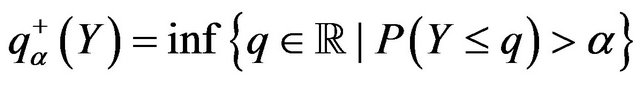 . For a random variable having continuous and strictly increasing distributions function
 ,
,
 , i.e. it solves the equation
 .
.
Here we take the portfolio loss  to describe a financial position in a fixed time interval and, in order to simplify notations, we assume in this section that
  has a continuous and strictly increasing distributions function. The Value-at-Risk at level
  is defined as

Let  be the value of the risky asset,
  and
and  be the risk-free rate, that without loss of generality we consider fixed in the period: we define the loss at time
  of such a position as
  implying
 . Let us now consider a classical hedging problem in which an institution has an exposure to a risky asset
  and decide to hedge such an exposure in the interval
  by buying a fraction
  of an European put option on the asset with maturity T and strike price K. Analogously to the situation considered in [1], we take as the hedged position the portfolio composed by the risky asset and the put option: the loss of the hedged portfolio at time
  is therefore
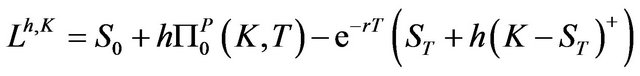 where
where  is the price of the put option at time
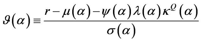
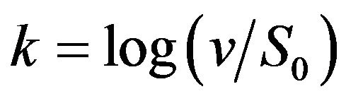
 . By defining the strictly increasing function
 , where
 , it is immediately seen that
 ; therefore

Let us firstly notice that if , then
 since
since . Hencegiven the budget constraint C, the optimal hedging strategy is specified by the following problem:

(1)
Since , the optimality first order condition for
  is given by the following non-linear equation:
 (2)
(2)
Assuming that (2) has a solution  and the twice differentiability of the price functional we can prove that this is actually a minimum since
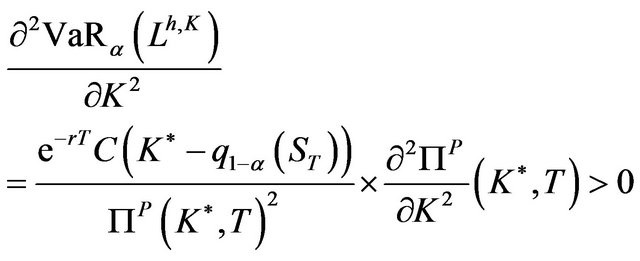
by the convexity of the price functional w.r.t. the strike. Correspondingly, the optimal amount of the hedging put option is
 (3)
(3)
We now assume the following:
Assumption 2.1. The price of the put option can be represented as the discounted expected value of the payoff at time  under a risk-neutral measure
 :
:

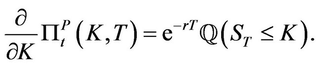
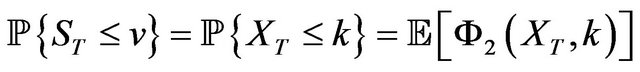
Furthermore, let  be the cumulative distribution function (cdf) of the random variable
  under such a measure: hence

and
We can finally prove the following property:
Proposition 2.1. If , then
 .
.
Proof. Since  and
and  are characterized through (2) and (3), we get
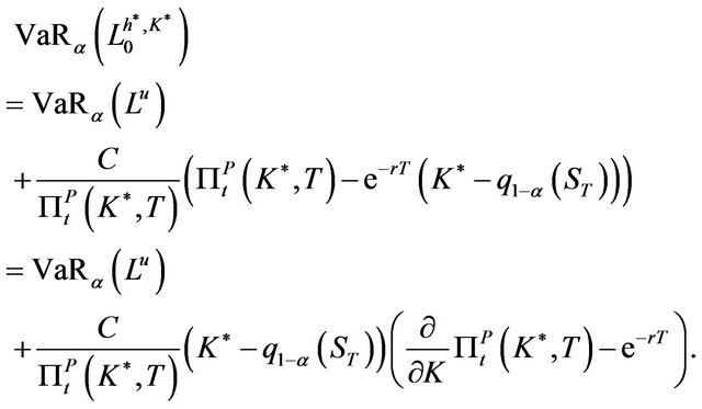
From Assumption 2.1, we have
 .
.
Therefore

Remark 2.1. Notice that the optimality condition (2) under Assumption 2.1 simplifies to
 (4)
(4)
and depends on both the objective and the risk neutral distributions  and
and . Furthermore, it easily seen that the l.h.s. is equal to the conditional expectation
 which is an increasing function of K bounded by
 . Therefore, (4) has a unique solution if and only if
 .
.
3. Regime-Switching Jump Diffusions and Measure Change
Let us consider on a filtered probability space
 a stochastic process of the form
 ,
,  , modeling the value, of a risky asset for
 . We consider a jump-diffusion setting in which the jump process is described as a marked point process (MPP), that is a random measure
  characterized by the intensity process
 , the parameters of which are driven by a finite state and continuous time Markov chain. So, let
  be a continuous time, homogeneous and stationary Markov Chain on the state space
  with generator
 : the elements
  of the matrix
 are positive numbers such that
 , for
, for
 . Furthermore,
  ,
,  and
and  are given functions,
  being the measurable mark space. Without loss of generality, we can assume in the following
 . In a given interval
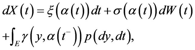
 , we consider the dynamic
(5)
where  is a standard brownian motion and
  is a MPP characterized by the intensity
 . Here
  represents the (regime-switching) intensity of the Poisson process
 , while
  are a set of probability measures on
 , one for each state (regime)
 . The function
  represents the jump amplitude relative to the mark
  in regime
 . The couple
  is called the
 -local characteristic of
 .
.
Furthermore  is a martingale for a suitable class of processes
  (see [14]),
being the compensated process.
Throughout the paper we assume that the processes  and
and  are independent,
  and
and  are conditionally independent given
  and that
 is finite for each regime
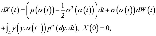
 . An application of the generalized Ito’s Formula gives the corresponding jump-diffusion SDE for the asset price
 (6)
(6)
with  and
and .
.
Measure changes. An absolutely continuous transformation of measures in a jump-diffusion setting allows to change the intensities of the MPP and the Markov chain in addition to the translation of the Wiener process (see [14]). It results convenient to represent the underlying Markov chain itself as the MPP  with finite mark space
 ,
,
 and
and : the compensator is
 (7)
(7)
 being the Dirac measure. Consequently, let
 be a square integrable predictable processes,
 a non-negative function such that
 and let
  and
and
 be strictly positive functions defined on
  and
and , respectively. We can define a new measure
  on the measurable space by setting
 (8)
(8)
Besides the translation of the Wiener process , we perform a change in the intensity of the MPP giving the compensated process
  with
with  -local characteristic (
 ,
, ) and a change of the intensity of the Markov chain which under
  has generator
  where
where

By taking the Radon-Nikodym derivative
 (9)
(9)
and supposing that  for
for , we have a probability measure
  on
on  equivalent to
  with
with , under which
 (10)
(10)
where  (see [14]).
In order to price derivatives under the model (6) we need to specify a risk-neutral or martingale measure, that is a measure under which the discounted price process  is a martingale. This is done by taking
 (11)
(11)
from which we finally get the risk-neutral dynamic for the underlying
 (12)
(12)
Correspondingly, for the process  we have
 (13)
(13)
The measure transformation defined by (8) through (9) preserves the probability structure of the stochastic process  under both
  and
and . It worth noting that we can specify infinitely many equivalent measures
 . In practice, the usual way to select one of the equivalent measures is to calibrate the model to a set of observed data.
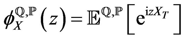
GFT for regime-switching jump-diffusions. In order to apply Fourier methods, we need to calculate the Fourier transform  of our process. Since we have to consider the process
  under two different measure, we derive its characteristic function for the following general dynamic
 (14)
(14)
with  local characteristic, and Markov chain generator
 . In [8] it was proved the following Proposition 3.1. Let
  be the generalized Fourier transform of the jump magnitude under the given measure. Then, by letting
 (15)
(15)
and , we have
 (16)
(16)
where ,
,
 and
and  is the transpose of Q.■
Different models can be recovered with simple linear constraints on the full parameter set of our model (RSJDM) (6), (12),  ,
, . This follows by noticing that if
 ,
,
 and
and  we are implicitly assuming a unique regime so recovering the well-known characteristic function of the (single-regime) jump-diffusion dynamic
which includes the standard geometrical Brownian motion (GBM) , the Merton jump-diffusion models (JDM); furthermore, if
  we get the regimeswitching version of GBM (RSGBM).
The evaluation of the characteristic function requires to compute matrix exponentials for which efficient numerical techniques are available; conversely, the case  can be considered explicitly (see [8] and the references therein).
4. Computing Results
In order to implement the optimal hedging strategy, we need to evaluate the VaR of the risky asset and the value of a put option. Both steps can be efficiently faced by means of Fourier methods. In this section we firstly outline such a technique and then we apply it to study numerically a model with two regimes and gaussian jumps.
4.1. Fourier Methods
Fourier transform methods are efficient techniques emerged in recent years as one of the main methodology for the evaluation of derivatives. Here we consider the technique introduced in [15] which consider the generalized Fourier transform with respect to the trigger parameter characterizing the payoff.
More formally, let  be the payoff at maturity of the derivative: for example,
  is the payoff of the put option. The no-arbitrage price is therefore given by

Due to the exponential structure of the underlying dynamic , it is convenient to represent the payoff with respect to the new variables
  and
and , in such a way
 .
.
Therefore, let us denote with  an arbitrary payoff function and with
  its generalized Fourier transform (GFT) w.r.t.
 , that is

under proper regularity conditions about the payoff and the Fourier transform of the underlying dynamic variables (see e.g. [16]), it can be proved that

in some strip of . Let us consider the payoff functions
 , and
, and , in such a way
  and
and
 , with
 . Their GFT w.r.t. the trigger parameter
  are
are

respectively. Hence we get the formulas
 (17)
(17)
and

(18)
 being the (generalized) Fourier transform, or characteristic function, of the random variable
  under the appropriate measure. If this is a regular functions in a properly defined strip of
 , the transform method can be applied in both cases (see [16]). Since under the Assumption (2.1) the optimality condition is

the optimal hedging strategy is then implemented by running twice a root search algorithm to find the values 1)  such that
 (19)
(19)
2)  such that

(20)
Numerical quadrature must be used for integral evaluation. Alternatively the FFT algorithm can be used to efficiently approximate integrals (see [16]) and then a standard root-finding routine will find the required solutions.
4.2. Some Numerical Results
We report some numerical results about the valuation of the optimal hedging strategy in the regime-switching jump-diffusion framework. An extended set of results can be found in [17]. All numerical procedures were implemented in the MatLab© framework. A standard rootsearch algorithm was used to solve Equations (19) and (20), with  and
and , together with the GaussLobatto quadrature for approximating the corresponding integrals. Few milliseconds were needed to get the required quantities on an Intel© Core i5.
We consider a two-state regime switching version of the jump-diffusion model with gaussian jumps
 ,
,  , characterized by the parameters
  and
and . The two state Markov chain
  has generator
 .
.
The first issue we consider is the reduction of risk obtained by implementing the optimal hedging strategy in the RSJD framework. The risk reduction percentage
 evaluated for different set of parameters range from 4.39% up to 58%, meaning that the strategy is effective in reducing the portfolio VaR, even in presence of jumps and regime-switching. On the other hand, by changing the value of some relevant parameters inside each model (GBM, JD, RSGBM, RSJD) the profile of the hedging portfolio VaR can change significantly. Hence we face the following issue: what is the effect of a wrong model specification which discards regime switchings and jumps, when they are indeed present in the market, and consider the simpler GBM model? In order to explore the model sensitivity of the optimal hedging strategy, we implemented the following exercise. We firstly fixed a RSJD model by choosing a complete set of parameters. Then we generated a set of call/put prices on which we calibrate the GBM model, finding the volatility
  with a constrained non-linear leastsquares algorithm: hence we run the optimal hedging strategy obtaining
  and correspondingly the minimal VaR,
 . We finally calculated the probability

under the RSJD model. This step requires to evaluate the integral in (18): as before, we use a Gauss-Lobatto quadrature algorithm. Results are shown in Tables 1 and 2.
Table 1. Optimal hedging strategy  under the simulated true model (first column), the fitted GBM model (second column—estimated volatility) and the corresponding value of
 . Here
 ,
,  ,
,  ,
,  ,
,  ,
,  ,
,  ,
,  ,
,  ,
, ; furthermore
 ,
,  and the budget constraint is
 .
.

Table 2. Optimal hedging strategy  under the simulated true model (first column), the fitted GBM model (second column—estimated volatility) and the corresponding value of
 . Here
 ,
,  ,
,  ,
,  ,
,  ,
,  ,
,  ,
,  ,
,  ,
, ; furthermore
 ,
,  and the budget constraint is
 .
.

Table 3. Optimal hedging strategy  under the simulated true model (first column), the fitted GBM model (second column—estimated volatility) and the corresponding value of
 . Here
 ,
,  ,
,  ,
,  ,
,  ,
,  ,
,  ,
,  ,
,  ,
, ; furthermore
 ,
,  and the budget constraint is
 .
.

Notice that even when the optimal strategies are similar, the probability that the portfolio loss exceeds the (optimal) VaR is greater than the fixed level . Of course this behavior depends on the choice of the parameters, but the underestimation produced by a wrong model choice can be quite severe: see Table 3, where parameters from a real data set were used (see [8]).