Concatenated Processes in Commercial Business and in Global Economy ()
1. Introduction
The tool that will be used at solution is the theory of Markov’s processes. It can be applied in some scientific areas and also in technological and economical branches. Formulae of this theory in stable state are well known. They are used for calculation of service channels like cash desks in department stores, seats in canteens, workplaces in call centres or help desks. The results of the theory in stable state are widely used especially in telecommunication praxis at dimensioning of communication channels and switching nodes. But less known are results of this theory in transition (non stable) state. Some examples can be taken from nuclear physic, boilogy and radio communication [1,2]. The theory describing random processes in transition state can also be applied on the special problem as indicated below.
2. Deterministic Case
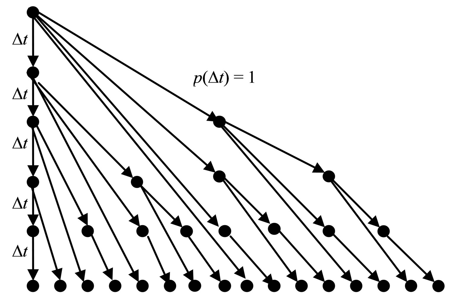
Let’s have an element that is able to augment itself once with the certainty (with probability equal to 1) in each time interval Dt in average. Its descendants have also the same ability. In this way, there will be 1 element born in the 1st time interval, 2 elements in the 2nd time interval, and 4 elements in the 3rd time interval, etc. (Figure 1). The number of elements born in the k-th time interval will be:

The entire count of elements after k time intervals will be:

Figure 1. Simple deterministic concatenated process.
 (1)
(1)
as Equation (1) performs the geometrical series.
As it is evident from Equation (1) and Figure 1 it is a simple concatenated process which quickly grows over any limits. Here is an example of an ideal concatenated process.
Let’s imagine a simple business model. A person who initially starts the business builds a net of agents (dealers, vendors) and clients in order to sell special goods or to render insurance or financial advices. He acquires 1 subject in each time interval in average (during a day, a week, a month or even a year). The gradually acquired new subjects do the same. As soon as a new subject acquires a new client, this subject becomes the agent. The agents continue gaining other clients and so one. When k time intervals elapse, there will be n subjects. In that manner the pyramidal structure grows. Thus after k time steps, there will be  clients on the bottom of the structure,
  subjects who are agents, and finally 1 agent-founder of the pyramidal business, together n/2 clients and n/2 agents. The clients on the bottom of the concatenated pyramid pay money for delivered goods or rendered services. The payments are distributed among agents. The higher an agent is in the pyramid, the higher incomes he has because he cashes money not only from his client, but he gets a certain part of money from his subordinated agents. The chief of the business on the top of the pyramid cashes the most of money as he has the most subordinated agents and he need not pay any money to anybody. The business will prosper only on condition when clients either pay once for 1 piece of goods or 1 piece of advice, but in this case the net must be increased step by step, or clients must constantly pay for rendered services and their number must not decrease. Otherwise, the business will cease.
Such situation cannot happen in real life because the indicated example is idealistic. It does not take into account the real conditions, e.g. acquisition of new clients in the business based on the pyramidal structure cannot continue permanently because the number of inhabitants on disposal in a country is finite. Acquisitions proceed with a certain probability and members of the business may also leave it due to the fact they have no interest to take part in the business more or they simply die.
Therefore a more perfect mathematical toll has to be used for solution of above cases occurring in real life.
3. Stochastic Case
3.1. General Mathematical Specifications
The used mathematical tool is the theory of Markov’s processes. In order to explain the problem more clearly and more comprehensive, we avoid the complex description of Markov’s processes in matrix form, as it is presented in special mathematical textbooks [3-5]. Instead of it the non-matrix descriptions adapted on the particular case will be used and constraining conditions will be defined.
Formula for the full probability is fundamental for our further considerations (refer also to [6]):
 (2)
(2)
Here P{A} is probability of an appearance A which can only occur together with appearances Aj that create the full set of mutually excluding appearances and therefore the sum of their probabilities P{Aj} for all j = 0, 1, 2, ···, n, ··· must be equal to 1. P{A/Aj} is the conditional probability with which the appearance A occurs together with one of appearances Aj.
Let’s consider a system that actually (in time t) contains k elements. Further let denote:
l—number of elements having entered (appeared in) the system during a time unit;
m—number of elements having left the system during a time unit;
n—entire number of elements that the system may achieve;
t = 1/m—average time an element stays in the system;
t—time;
Dt—time interval;
pj(t)—probability the system contains j elements in a time t;
pk(t + Dt)—probability the system will contain k elements in a future time t + Dt;
pj,k(Dt)—conditional probability the system transits from the status having j elements to the status having k elements within an arbitrary short time interval Dt®0;
P—cumulative probability in a given range.
Only from pure practical reasons, let the ratio
 (3)
(3)
denote a growing factor (a > 1) or eventually a sinking factor (a < 1) and
 (4)
(4)
denote a relative time.
The constraining conditions are as follows:
• Entering of elements into the system and their leaving out of the system is not controlled in any manner, but they are fully random.
• No more than 1 change is allowed in the system during an arbitrary short time interval Dt®0, i.e. just 1 element may enter or leave the system, or the system stays without any change during the time interval Dt.
• The probabilities pj,k(Dt) proportionally depend only on the time interval Dt and they do not depend on where on the time axis, t the time interval Dt lays (they are time invariant). Also the constants l and m are time invariant.
Issuing from these fundamental conditions, the basic equations can be set up.
3.2. Growth and Ceasing Process
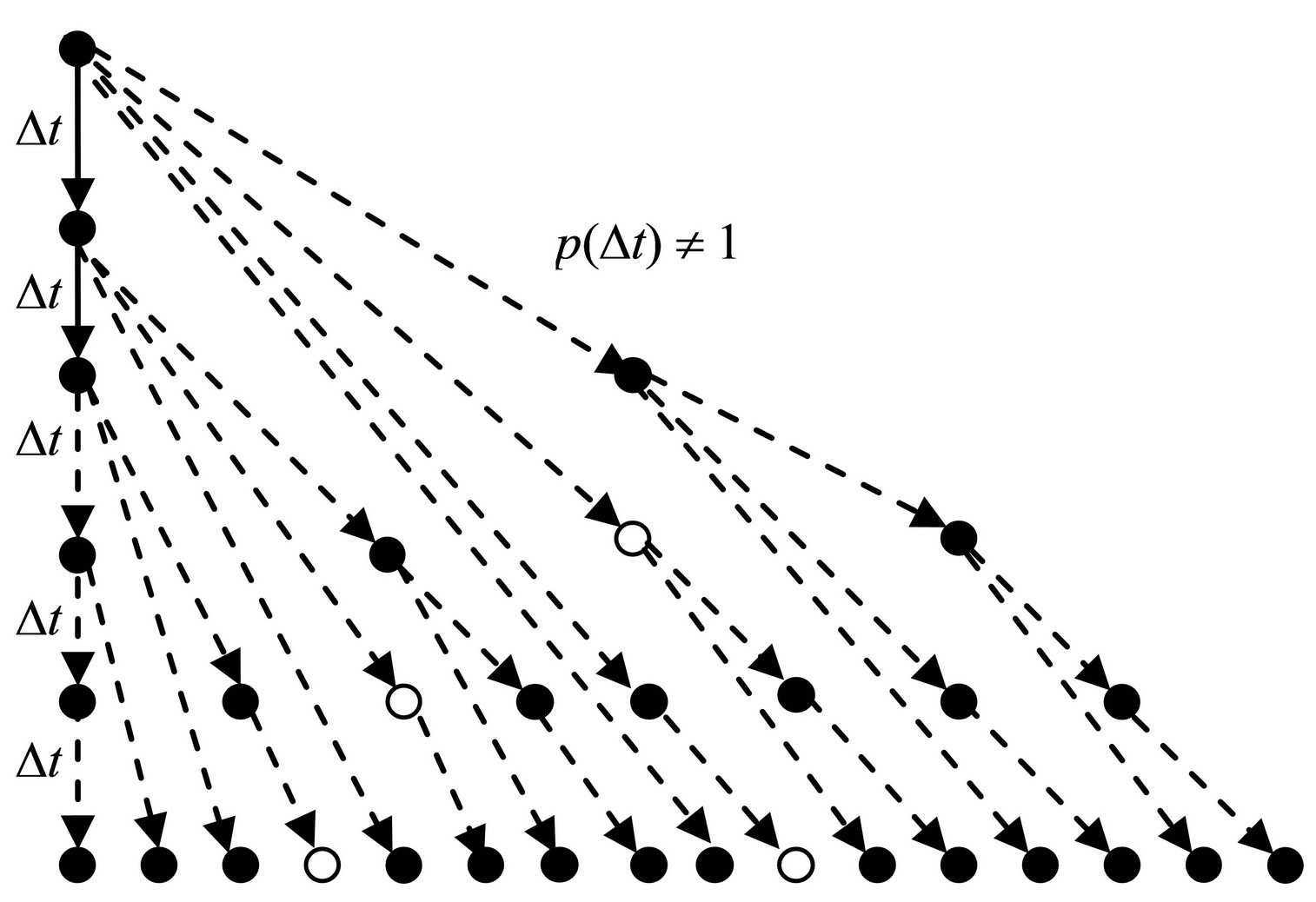
Let’s consider the system performed by the concatenated pyramidal structure as in Figure 2. The elements in the system are able to augment themselves with a certain probability.The augmentation process means that new elements continuously and randomly enter the system.

Figure 2. Stochastic growth and ceasing concatenated process.
Moreover, some of the elements may also leave the system continuously and randomly with another probability after a certain time (which is indicated by empty little circles in Figure 2). Therefore a limitation of the count of elements in the system need not be taken into account in this case.
Theoretic Background
Keeping on mind the fundamental conditions, there are 3 possibilities how the system can get to the state with k elements in a future time t + Dt:
• either just 1 element enters the system containing  elements during Dt probability of which is
 ;
;
• or no element neither enters nor leaves the system containing k elements during Dt probability of which is ;
;
• or just 1 element leaves the system containing k + 1 elements during Dt probability of which is .
.
Issuing from the formula for the full probability (2) we can write for the considered system:
 (5)
(5)
It is assumed that the transition probability,  is proportional to the number of elements,
  being in the system in an actual time, t and to the entering intensity, l:
 (6)
(6)
Similarly, the transition probability pk + 1,k(Dt) is also proportional to the number of elements still being in the system, k + 1 and to the leaving intensity, m:
 (7)
(7)
when the system contains k elements in an actual time, t and it shall stay in the same state in a future time, t + Dt, no element must enter or leave the system during Dt:
 (8)
(8)
In other words, when an element comes into being, it may bear other elements during its being in the system. Each other new born element may do the same. The more elements exist in the system, the higher the probability of their birth is and also the higher the probability of their deaths.
Now we can return to Equation (5) having put Equations (6)-(8) into it:


We have obtained the system of the infinite number of differential equations:

To solve this system, the next operation shall be applied on it:

 (9)
(9)
These necessary modifications have to be made:


Putting these modifications into (9) we will have:
 (10)
(10)
The term
 (11)
(11)
is the generation function. Applying it on Equation (10) we obtain the partial differential equation:

And finally:

It is the linear homogenous partial differential equation of type:

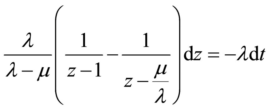
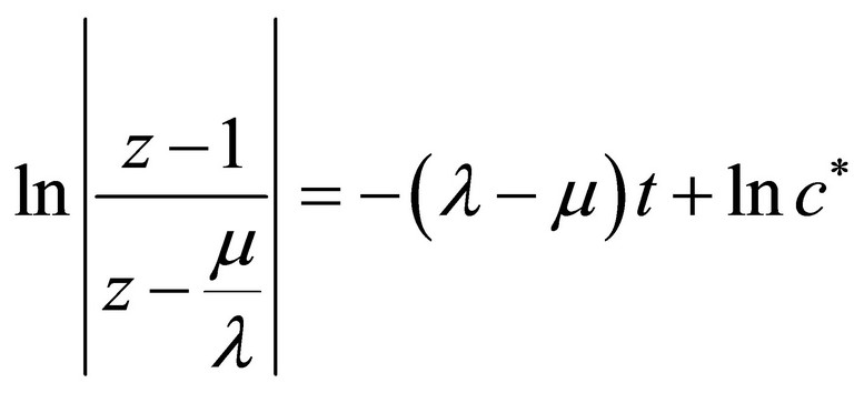
Solution of this equation can be transferred to solution of the system of the common differential equation in the next canonical form [4]:

where:


 (12)
(12)
Here c’, c*, c are arbitrary integration constants.
Let z = z0 for t = 0 and according to (11)
 (13)
(13)
as on the beginning when t = 0 the system started withn elements in a general case probability of which is 1. When there is only 1 element at the beginning, then n = 1. Replacing the time variable, t by 0, constant c will be determined:
 (14)
(14)
Replacing constant c in (12) by (14) we have:

The variable z0 shall be expressed from this equation:

because it is the sought generation function f (t, z) at the same time according to (13).
The next effort will be to make such mathematical arrangements that will lead to the geometrical series that will correspond with the generation function (11). The last equation will be arranged as follows:

Let
 (15)
(15)
where the terms (3) and (4) were also used. From there:


 (16)
(16)
The term in Equation (16) corresponds with the generation function (11). Comparing these we have:
 (17)
(17)
 (18)
(18)
Using the terms (3) and (4):
 (19)
(19)
 (20)
(20)
The terms (17) and (18) perform the probability distribution and therefore

The stable state will become when x®¥. Putting it to (19) there will be:
 (21)
(21)

Though the intensity of entering elements prevails the intensity of leaving elements (the growth factor a > 1), it can happen the system will get empty with a probability p0, which is evident from (21).
As it can be seen from Figure 3, probability the concatenated structure will ever cease is relatively high at low values of a. For the balanced case, when a = 1
 (22)
(22)
and the structure would cease with probability of 0.95 after 20 time units (here 1 time unit means the average time an element stays in the system).
Probability there are up to n elements in the system is:

No matter of how many elements, n exist in the system, the probability Pn(x) converges to:

and in the limit case:

4. Conclusions
It would seem that the business based on a concatenated pyramidal structure can only crash when the count of new acquired members, l will be lower than the count of members they left the structure, m. This is not true. There is always a certain probability, p0 the business will cease even if the count of new members acquired, l is higher than the count of members, m they left the structure. This
probability is the highest in case when these numbers are balanced (a = 1) [see (21) and (22)] and the business will certainly crash after a longer time (theoretically in time t®¥). The probability the business will cease decreases when the growing factor, a increases. There will be a chance 50:50 the business sustains, only when the number of acquired members will be 2-times higher than the number of members they left the business. Therefore no person operating the business based on such concatenated structure can be sure that the business will last for ever. The founder and his agents must take high effort to maintain the business and therefore they must always acquire new and new clients.
The global economic is a great business. It is also based on the structure similar to that as described above. Large international corporations perform associations of big national companies which affiliate smaller enterprises and these enterprises have its own suppliers that provide work occasions for many people. The motor car industry is a good example of such concatenated structure. Now let’s imagine that the economic growth would not be supported by implementation of discoveries, inventions, innovations issuing in technology development and the work productivity increase. It would have to rely only on the growth based on establishing of more new enterprises instead of perished ones. It would be hard to achieve the growth factor, a to be higher than 1 in the high developed countries like the USA, European Union, while the growth factor, a can be higher than 1 in less developed countries. But even if the count of new established enterprises is in 25% higher than perished ones (the growth factor a = 1.25), there would still be the probability of 80% that the economic will crash after a longer time [see (21)], if this growth is not supported by technology development. The times of great physical and industrial discoveries and inventions of the 20th century are over for ever. Today’s discoveries, inventions and innovations are mainly aimed on biology, genetic and health care and, in fact, they have not contributed to economic growth so far. These facts may be one of the reasons of today’s global economic problems in high developed countries.