A Comparative Study of Variational Iteration Method and He-Laplace Method ()
1. Introduction
Nonlinearity exists everywhere and nature is nonlinear in general. The search for a better and easy to use tool for the solution of nonlinear equations that illuminate the nonlinear phenomena of real life problems of science and engineering has recently received a continuing interest. Various methods, therefore, were proposed to find approximate solutions of nonlinear equations. Some of the classical analytic methods are Lyapunov’s artificial small parameter method [1], perturbation techniques [2,3],  -expansion method [4] and Hirota bilinear method [5-6]. In recent years, many authors have paid attention to study the solutions of nonlinear partial diffenential equations by using various methods. Among these are the Adomian decomposition method (ADM) [7], He’s Semiinverse method [8], the tanh method, homotopy perturbation method(HPM), Sinh-Cosh method, the differential transform method and the variational iteration method (VIM) [9-17]. Several techniques including the Adomian decomposition method, the variational iteration method, the weighted finite difference techniques and the Laplace decomposition method have been used to solve nonlinear differential equations [18-26]. J. H. He developed the homotopy perturbation method (HPM) [27-42] by merging the standard homotopy and perturbation for solving various physical problems. The Laplace transform is totally incapable of handling nonlinear equations because of the difficulties that are caused by the nonlinear terms. Various ways have been proposed recently to deal with these nonlinearities such as the Adomian decomposition method [43] and the Laplace decomposition algorithm [44-48]. Furthermore, the homotopy perturbation method is also combined with the well-known Laplace transformation method [49] which is known as He-Laplace method.
In this paper, the main objective is to introduce a comparative study to nonlinear ordinary differential equation and partial differential equations by using variational iteration method and He-Laplace method.
It is worth mentioning that He-Laplace method is an elegant combination of the Laplace transformation, the homotopy perturbation method and He’s polynomials. The use of He’s polynomials in the nonlinear term was first introduced by Ghorbani [50]. The proposed algorithm provides the solution in a rapid convergent series which may lead to the solution in a closed form. This paper contains basic idea of homotopy perturbation method in Section 2, variational iteration method in Section 3, Laplace homotopy perturbation method in Section 4 and conclusions in Section 5 respectively.
2. Basic Idea of Homotopy Perturbation Method and He-Laplace Method
2.1. Homotopy Perturbation Method
Consider the following nonlinear differential equation
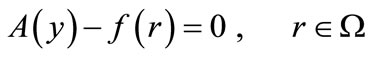 (1)
(1)
with the boundary conditions of
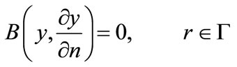 (2)
(2)
where A, B,  and
and  are a general differential operator, a boundary operator, a known analytic function and the boundary of the domain
 , respectively.
The operator A can generally be divided into a linear part L and a nonlinear part N. Equation (1) may therefore be written as:
 (3)
(3)
By the homotopy technique, we construct a homotopy  which satisfies:
 (4)
(4)
or
 (5)
(5)
where  is an embedding parameter, while
  is an initial approximation of Equation (1), which satisfies the boundary conditions. Obviously, from Equatons (4) and (5), we will have:
 (6)
(6)
 (7)
(7)
The changing process of p from zero to unity is just that of v(r, p) from y0 to y(r). In topology, this is called deformation, while  and
and  are called homotopy. If the embedding parameter p is considered as a small parameter, applying the classical perturbation technique, we can assume that the solution of Equations (4) and (5) can be written as a power series in
 :
:
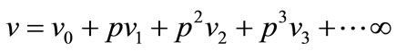 (8)
(8)
Setting  in Equation (8), we have
 (9)
(9)
The combination of the perturbation method and the homotopy method is called the HPM, which eliminates the drawbacks of the traditional perturbation methods while keeping all its advantages. The series (9) is convergent for most cases. However, the convergent rate depends on the nonlinear operator . Moreover, He [51] made the following suggestions:
1) The second derivative of  with respect to
  must be small because the parameter may be relatively large, i.e.
 .
.
2) The norm of  must be smaller than one so that the series converges.
2.2. He-Laplace Method
Consider the following nonlinear differential equation (IVP):
 (10)
(10)
 (11)
(11)
where  are constants. f(y) is a nonlinear function and f(x) is the source term. Taking Laplace transformation (denoted throughout this paper by L) on both side of Equation (10), we have
 (12)
(12)
By using linearity of Laplace transformation, the result is
 (13)
(13)
Applying the formula on Laplace transform, we obtain
 (14)
(14)
Using initial conditions in Equation (14), we have
 (15)
(15)
or
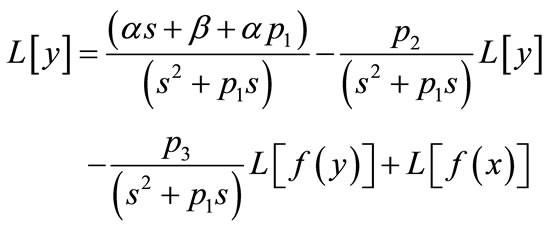 (16)
(16)
Taking inverse Laplace transform, we have
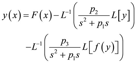 (17)
(17)
where  represents the term arising from the source term and the prescribed initial conditions.
Now, we apply homotopy perturbation method [51],
 (18)
(18)
where the term  are to recursively calculated and the nonlinear term
  can be decomposed as
 (19)
(19)
for some He’s polynomial  (see [50,52]) that are given by

Substituting Equations (18) and (19) in (17), we get
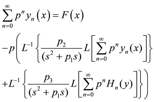 (20)
(20)
which is the coupling of the Laplace transformation and the homotopy perturbation method using He’s polynomials. Comparing the coefficient of like powers of p, the following approximations are obtained:
 (21)
(21)

Example 2.1. Consider the following nonlinear PDE [53]:
 (22)
(22)
with the following conditions:
 (23)
(23)
Equation (22) can be written as
 (24)
(24)
By applying the Laplace transform to both sides of Equation (24) subject to the initial condition, we have
 (25)
(25)
The inverse of the Laplace transform implies that
 (26)
(26)
Now, we apply the homotopy perturbation method, we have
 (27)
(27)
where  are He’s polynomials. The first few components of He’s polynomials are given by
 (28)
(28)
Comparing the coefficient of like powers of p, we have
 , but we consider
 (29)
(29)
So that the solution  is given by
 (30)
(30)
which is the exact solution of the problem.
Example 2.2. Consider the following non-homogeneous nonlinear PDE [53]:
 (31)
(31)
with the following condition:
 (32)
(32)
By applying the Laplace transform method subject to the initial condition, we have
 (33)
(33)
The inverse of the Laplace transform implies that
 (34)
(34)
Now, we apply the homotopy perturbation method, we have
 (35)
(35)
where  are He’s polynomials. The first few components of He’s polynomials are given by
 (36)
(36)
Comparing the coefficient of like powers of p, we have
 (37)
(37)
Proceeding in a similar manner, we have


So that the solution  is given by
 (38)
(38)
3. Variational Iteration Method (VIM)
To illustrate the basic concept of the technique, we consider the following general differential equation

where L is a linear operator, N is a nonlinear operator and g(x) is the forcing term. According to VIM, we can construct a correct functional as follows

where  is a Lagrange multiplier. The subscripts n denote the nth approximation,
  is considered as a restricted variation i.e.
 . In this method, it is required first to determine the Lagrange multiplier
  optimally. The successive approximation
  of the solution u will be readily obtained upon using the determined Lagrange multiplier and any selective function
 , consequently, the solution is given by
  .
.
Now, we consider the following examples:
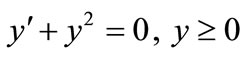
Example 3.1. Consider the following first order nonlinear differential equation [53]:
 (39)
(39)
 (40)
(40)
If  is an initial approximation or trial-function then we can write down following expression for correction:
 (41)
(41)
where the last term of right is called “correction”,  is a general Lagrange multiplier. The above functional is called correction functional, the Lagrange multiplier in the functional should be such chosen that its correction solution is superior to its initial approximation (trialfunction) and is the best within the flexibility of the trialfunction, accordingly we can identified the multiplier by variational theory [54,55]. Making the above correction functional stationary with y(0) = 1 so that, we can obtain following stationary conditions:
 (42)
(42)
 (43)
(43)
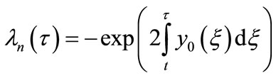
The Lagrange multiplier, therefore, can be identified as follows:
 (44)
(44)
To simplify the multiplier, we approximate Equation (44) as follows:
 (45)
(45)
Substituting Equation (45) in Equation (41) yields following variational iteration formula
 (46)
(46)
We start with by above iteration formula, we can obtain following results,
 (47)
(47)
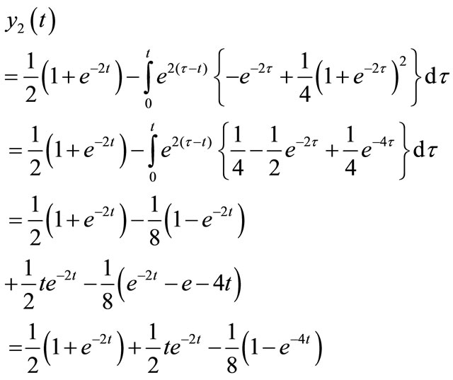 (48)
(48)
if, suppose,  is sufficient, the approximation at x = 0.4 is
 , while its exact one is y(0.4) = 0.6667, the 0.17% accuracy is remarkably good in view of the crudeness of its initial approximation. The process can, in principle, be continued as far as desired, however, the resulting integrals quickly become very cumbersome, so some simplification in the process of identification of Lagrange multiplier will be discussed at below:
We re-consider the correction functional Equation (41) as follows:
 (49)
(49)
Where the nonlinear term  is considered as nonvariational variation or constrained variation [54], i.e.
  The Lagrange multiplier, therefore, can be readily identified and the following variation iteration formula can be obtained:
 (50)
(50)
Putting n = 0, 1, in Equation (50), we can obtain following results.

Similarly putting n = 2, 3, …, n − 1, the nth approximation can be obtained, which converges to its exact solution, a little more slowly due to the approximate identification of the Lagrange multiplier.
Remark
The variational iteration technique mentioned above can be readily extended to partial differential equations (PDEs). Here the author will illustrate its process.
Example 3.2. Consider the following equation [53]:
 (51)
(51)
which has the exact solution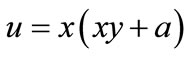 .
.
According to Adomian [56], an approximate solution can be obtained [57].
 (52)
(52)
It is obvious that the approximation does not satisfy its boundary conditions. In 1995, Liu [57] proposes a modified Adomian’s method called weighted residual decomposition method, with such method, he obtained following approximation:
 (53)
(53)
which satisfies all its boundary conditions and has more higher accuracy than Adomian’s. In 1978, Inokuti et al. [55] proposed a general Lagrange multiplier method to solve nonlinear mathematical physics which was first applied to quantum mechanics. In this method, a more accurate solution, depending upon its trial-function can be obtained for some special points, but not an approximate analytical one. J. H. He [53] tries to solve it by variational iteration method as follows:
Supposing the initial approximation of Equation (51) is , its correction variational functional in x-direction and y-direction can be expressed respectively as follows:
 (54)
(54)
 (55)
(55)
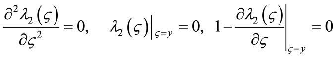
where  is a nonvariational variation. Their stationary conditions are written down respectively as follows
 (56)
(56)
and
 (57)
(57)
The Lagrange multipliers can be easily identified:
 (58)
(58)
The iteration formulae in x-direction and y-directions can be, therefore, expressed respectively as follows
 (59)
(59)
 (60)
(60)
To ensure the approximations satisfy the boundary conditions at x = 1 and y = 1, we modify the variational iteration formulae in x-direction and y-direction as follows:
 (61)
(61)
 (62)
(62)
Now we start with an arbitrary initial approximation: , where A and B are constants to be determined, by the variational iteration formula in x-direction (59), we have
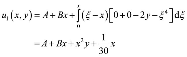 (63)
(63)
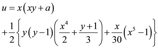
By imposing the boundary conditions at x = 0 and x = 1 yields A = 0 and B = a − 1/30, thus we have
 (64)
(64)
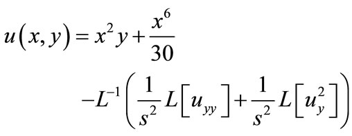
By (61), we have
 (65)
(65)
which is an exact solution. The approximation can also be obtained by y-direction.
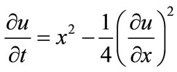
Example 3.3. Consider the following nonlinear PDE [53]:
 (66)
(66)

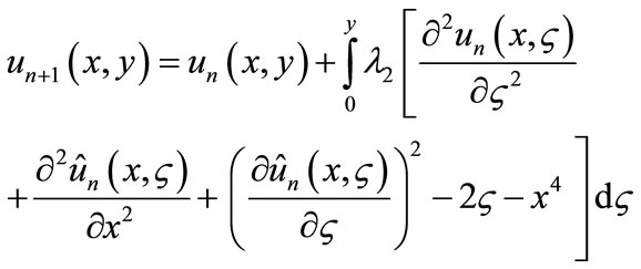
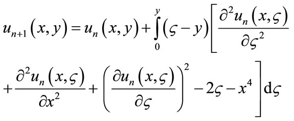
Its t-direction correction functional can be constructed as
 (67)
(67)
In which  is nonvariational variation. The multiplier can be identified and its variational iteration formula t-direction can be obtained
 (68)
(68)
We start with initial approximation  by above iteration formula, we can obtain successively its approximation:


which is the same as Adomian’s [56,58].
4. Comparision of Variational Iterational Method and He-Laplace Method
Example 4.1. Consider the following first order nonlinear differential equation [53]:
 (69)
(69)
with the following condition:
 (70)
(70)
By applying the aforesaid method subject to the initial condition, we have
 (71)
(71)
The inverse of the Laplace transform implies that
 (72)
(72)
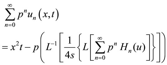
Now, we apply the homotopy perturbation method, we have
 (73)
(73)
where  are He’s polynomials. The first few components of He’s polynomials are given by
 (74)
(74)
Comparing the coefficient of like powers of p, we have
 (75)
(75)


Table 1. Numerical results of Example 4.1.
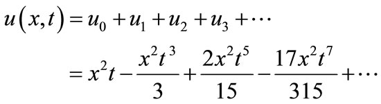
So that the solution  is given by
 (76)
(76)
which is converging to  i.e. exact solution.
The computational results are presented in Table 1.
5. Conclusion
In this paper, variational iteration method is employed for solving nonlinear ordinary and partial differential equations. The same problems are solved by He-Laplace method. It is worth mentioning that the He-Laplace method is capable of reducing the volume of the computational work as compared to the variational iteration methods while still maintaining the high accuracy of the numerical results.