Periodicity and Solution of Rational Recurrence Relation of Order Six ()

 where the initial conditions
  and
and  are arbitrary real numbers with
  and
and  not equal to be zero. On the other hand, we will study the local stability of the solutions of Equation (1). Moreover, we give graphically the behavior of some numerical examples for this difference equation with some initial conditions.
1. Introduction
Difference equations or discrete dynamical systems is diverse field whose impact almost every branch of pure and applied mathematics. Every dynamical system  determines a difference equation and vise versa. Recently, there has been great interest in studying difference equations. One of the reasons for this is a necessity for some techniques whose can be used in investigating equations arising in mathematical models decribing real life situations in population biology, economic, probability theory, genetics, psychology, ...etc. Difference equations usually describe the evolution of certain phenomenta over the course of time. Recently there are a lot of interest in studying the global attractivity, boundedness character the periodic nature, and giving the solution of nonlinear difference equations. Recently there has been a lot of interest in studying the boundedness character and the periodic nature of nonlinear difference equations. Difference equations have been studied in various branches of mathematics for a long time. First results in qualitative theory of such systems were obtained by Poincaré and Perron in the end of nineteenth and the beginning of twentieth centuries. For some results in this area, see for example [1-13].
Although difference equations are sometimes very simple in their forms, they are extremely difficult to understand throughly the behavior of their solutions.
Many researchers have investigated the behavior of the solution of difference equations for examples.
Cinar [1,2] investigated the solutions of the following difference equations


Karatas et al. [4] gave that the solution of the difference equation

G. Ladas, M. Kulenovic et al. [12] have studied period two solutions of the difference equation

Simsek et al. [13] obtained the solution of the difference equation

Ibrahim [5] studied the third order rational difference Equation

In this paper we obtain the solution and study the periodicity of the following difference equation
 , (1)
, (1)
 where the initial conditions


 , and
, and  are arbitrary real numbers with
 ,
,  and
and  not equal to be zero. On the other hand, we will study the local stability of the solutions of Equation (1). Moreover, we give graphically the behavior of some numerical examples for this difference equation with some initial conditions.
Here, we recall some notations and results which will be useful in our investigation.
Let I be some interval of real numbers and Let  be a continuously differentiable function. Then for every set of initial conditions
 , the difference equation
 (2)
(2)
has a unique solution  [11].
[11].
Definition (1.1) A point  is called an equilibrium point of Equation (2) if

That is,  for
for , is a solution of Equation (2), or equivalently,
  is a fixed point of F.
Definition (1.2) The difference Equation (2) is said to be persistence if there exist numbers m and M with 0 < m ≤ M < ∞ such that for any initial  there exists a positive integer N which depends on the initial conditions such that m ≤ xn ≤ M for all n ≥ N.
Definition (1.3) (Stability)
Let I be some interval of real numbers.
1) The equilibrium point  of Equation (2) is locally stable if for every ε > 0, there exists δ > 0 such that for
  with
with

we have  for all n ≥ −k.
2) The equilibrium point  of Equation (2) is locally asymptotically stable if
  is locally stable solution of Equation (2) and there exists γ > 0, such that for all
  with
with

we have 
3) The equilibrium point  of Equation (2) is global attractor if for all
 , we have
4) The equilibrium point  of Equation (2) is globally asymptotically stable if
  is locally stable, and
  is also a global attractor of Equation (2).
5) The equilibrium point  of Equation (2) is unstable if
  not locally stable.
The linearized equation of Equation (2) about the equilibrium  is the linear difference equation

Theorem (1.4) [10] Assume that  (real numbers) and
  Then
Then

is a sufficient condition for the asymptotic stability of the difference equation

Remark (1.5) Theorem (1.4) can be easily extended to a general linear equations of the form

where  (real numbers) and
 . Then Equation (4) is asymptotically stable provided that
 .
.
Definition (1.6) (Periodicity)
A sequence  is said to be periodic with period p if
  for all n ≥ −k.
2. Solution and Periodicity
In this section we give a specific form of the solutions of the difference Equation (1).
Theorem (2.1)
Let  be a solution of Equation (1). Then Equation (1) have all solutions and the solutions are

where .
.
Proof:
For n = 0 the result holds. Now suppose that n > 0 and that our assumption holds for n − 1. We shall show that the result holds for n. By using our assumption for n − 1, we have the following:

Now, it follows from Equation (1) that


similarly we can derive,

Thus, the proof is completed.
Theorem (2.2)
Suppose that  be a solution of Equation (1). Then all solutions of Equation (1) are periodic with period fourteen.
Proof:
From Equation (1), we see that

which completes the proof.
3. Stability of Solutions
In this section we study the local stability of the solutions of Equation (1).
Lemma (3.1)
Equation (1) have two equilibrium points which are 0 and 1.
Proof:
For the equilibrium points of Equation (1), we can write

Then , i.e.
Thus the equilibrium points of Equation (1) is are 0 and 1.
Theorem (3.2)
The equilibrium points  and
and  are unstable.
Proof:
We will prove the theorem at the equilibrium point  and the proof at the equilibrium point
  by the same way.
Let  be a continuous function defined by

Therefore it follows that


At the equilibrium point  we have
 ,
,  ,
,
 ,
,  ,
,
 ,
, 
Then the linearized equation of Equation (1) about  is
is

i.e.

Whose characteristic equation is

By the generalization of theorem (1.4) we have

which is impossible. This means that the equilibrium point  is unstable. Similarly, we can see that the equilibrium point
  is unstable.
4. Numerical Examples
For confirming the results of this section, we consider numerical examples which represent different types of solutions to Equation (1).
Example 4.1
Consider x−5 = 1, x−4 = 2, x−3 = 4, x−2 = −1, x−1 = −2, and x0 = 7. See Figure 1.
Example 4.2
Consider x−5 = 1, x−4 = −1, x−3 = 2, x−2 = −6, x−1 = 5, and x0 = −4. See Figure 2.
Example 4.3
Consider x−5 = 3, x−4 = 5, x−3 = −7, x−2 = −3, x−1 = 2, and x0 = −1. See Figure 3.
Example 4.4
Consider x−5 = −4, x−4 = 3, x−3 = −2, x−2 = 9, x−1 = 17,

Figure 1. The periodicity of solutions with period 14 with unstable equilibrium points  = 1 and
  = 0.
= 0.

Figure 2. Periodicity of solutions with period 14 with unstable equilibrium points  = 1,
= 1,  = 0.
= 0.

Figure 3. Periodicity of solutions with period 14 with unstable equilibrium points  = 1 and
  = 0.
= 0.
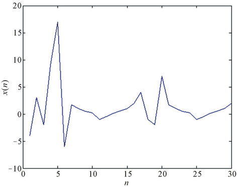
Figure 4. The periodicity of solutions with period 14 with unstable equilibrium points  = 1,
= 1,  = 0.
= 0.
and x0 = −6. See Figure 4.
5. Acknowledgements
We want to thank the referee for his useful suggestions.