An Accurate FFT-Based Algorithm for Bermudan Barrier Option Pricing ()
1. Introduction
Financial market is developing explosively, although it is struck by the financial tsunami recently. Many new financial derivatives, including options, warrants and swaps are springing out. They are widely used as risk management tool by investors, stock brokers and bankers. But still, options are the most popular derivative products as hedging tools in constructing a portfolio.
Since Bachelier, a French mathematician, first tried to give a mathematical definition for Brownian motion and used it to model the dynamics of stock process in 1900, financial mathematics has developed a lot. Many good ideas have been proposed to model the stock pricing processes since then. Recently serval exponential Lévy models are used to model financial markets. For example, Merton’s model, Kou’s model, Variance Gamma (VG) model, Inverse Gaussian (IG) model, Normal Inverse Gaussian (NIG) model, and CGMY model, etc. (refer to [1-5]). Meanwhile, many efficient numerical methods for option pricing have been proposed. These methods can be classified into three major groups: numerical solutions to partial integro-differential equations (PIDEs), Monte Carlo simulation techniques, and numerical integration methods. Each of them has its advantages and disadvantages for different financial models and specific applications (refer to [6]).
This paper concerns with the application of numerical integration methods to price a Bermudan barrier option. A Bermudan option is an option where the buyer has the right to exercise at a set of pre-specified exercise dates before the maturity. A barrier option can either come into existence or become worthless if the underlying asset reaches a prescribed level (known as barrier) before the maturity.
Pricing Bermudan or barrier options is much harder than pricing European options. Because these options are depended on paths of the price process for the underlying assets. Recently, some new numerical integration methods based on Fourier transforms are proposed. An efficient and accurate FFT-based method, called the CONV method, was presented by Lord et al. to price Bermudan options in [2]. A fast Hilbert transform approach was considered by Feng and Linetsky to price barrier options in [7]. And a novel numerical method based on Fouriercosine series expansion, called the COS method, was proposed by Fang and Oosterlee to to price Bermudan options and barrier options respectively (refer to [8,9]). This method was also extended to price Bermudan barrier options in [10].
In this paper, the CONV method is applied to price the Bermudan barrier option in which the pre-specified monitored dates may be many times more than the prespecified exercise dates. The corresponding numerical algorithm is presented for practical option pricing. This algorithm works very well and accurately for different exponential Lévy asset models. Numerical experiments on this algorithm are also given to support the accuracy of this algorithm.
This paper is structured as follows. After this introduction, the CONV method is applied to derive the approximate pricing formula for Bermudan barrier options under the exponential Lévy asset models in Section 2. Then, the corresponding numerical algorithm is presented for practical Bermuda barrier option pricing in Section 3. Finally, the practical Bermudan barrier option prices are computed by numerical experiments under the geometric Brownian motion (GBM) model and the CGMY model, respectively, in Section 4.
2. The CONV Method
Let T be the maturity of the option considered here, and let M and L be two given positive integers. Denote

the set of pre-specified monitored dates before the maturity , and
, and

the set of pre-specified exercise dates before the maturity , where
with  for any
 . We consider an American barrier option , which is discretely monitored at every
  and can be exercised at each
 , namely Bermudan barrier option, whose payoff is given by

Here  for a call and
  for a put with the strike price
  and the spot price
 , and
, and  is the price of the underlaying asset at time
 , and
, and  is the constant barrier. Thus, this is an up-and-out Bermudan barrier option.
Assume that, under the risk-neutral probability, the price of the underlaying asset is given by

where  is a Lévy process and
  is the initial price. For instance, in the GBM model,
  is given by

where  is a standard Brownian motion; in the CGMY model,
  is a CGMY process. The detail of these exponential Lévy models can be found in [4]. Let
  be the conditional density of
  given
given  for
for  under the risk-neutral probability. Set
 (1)
(1)
and denote  as the option price for the spot stock price
 . Then, it is clear that
 (2)
(2)
where . With help of the risk-neutral valuation, the option price can be computed recursively by the backward induction: letting
 (3)
(3)
for each , and then, if
 ,
,
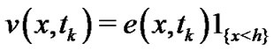 (4)
(4)
and if 
 (5)
(5)
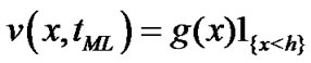
Finally, the option price  is given by
 (6)
(6)
Since each Lévy process is stationary and has independent increments, the conditional density  possesses the property:

where  is the density of
 . Applying this property infinite integrals
  in (3) becomes to
 (7)
(7)
for any . Then, the integral (7) can be rewritten as a convolution of
  and the function
 , i.e.
 (8)
(8)
Thus, for any , we have

Now, the main idea of the CONV method, which was proposed by Lord et al. in [1], is that, taking the Fourier transform in the both sides of the above equation and applying the Convolution theorem of Fourier transform, the integral becomes

where  is the the Fourier transform of function
 , i.e.

Here  is the imaginary unit. Denote
 ,
,  , is the characteristic function of the density
  on the complex plan
 , i.e.

Then, by a simple calculation, we have

Thus, taking the inverse Fourier transform we obtain
 (9)
(9)
Now, by employing the fast Fourier transform (FFT), the integral  can be fast and accurately approximated by the numerical integrals in (9).
3. The Numerical Algorithm
Denote
 (10)
(10)
where  is the characteristic function of
 , and
, and  is a proportionality constant, which is taken as
  for the GBM model and
  for other exponential Lévy models according to the suggestion from [1]. Let
  be an even integer. We consider the grid points on
  -axes:

where . Furthermore, we also consider the grid points for the numerical integrals in (9):

where . It is clear that these grids satisfy the Nyquist relation:
 . Now, for each
  and each
 , approximating the first integral in (9) with composite trapezoidal rule and the second integral with left rectangle rule yields

where the weights  are chosen as
and  for
for . Noting that
 and
and , we have
 (11)
(11)
Therefore, we can use FFT to calculate the summations in the right side of (11). In fact, using the notations of the discrete Fourier transformation (DFT) and the inverse discrete transform (IDFT), we have
 (12)
(12)
where

and

are the DFT of sequence  and the IDFT of sequence
 .
.
Once the integral  is computed by (11), we can determine the early-exercise price
 ,
,  , by the procedure: for each
 , locate
  such that
 (13)
(13)
or,
 (14)
(14)
In the case (13) set , and in the case (14)
set . Then the early-exercise price at every
  is given by
 .
.
We summarize the practical pricing procedure by the following algorithm:
Algorithm: (Price an up-and-out Bermudan barrier option.)
1) Calculate ,
,  by the formula:

2) Take the following backward induction for  :
:
a) For each , compute
 ,
,  , by the formula (12), and calculate
 ,
,  by the formula:

until  then go to Step b).
b) For each , compute
 ,
,  , by the formula (12), and determine the early-exercise price
 . Then, calculate
 ,
,  by the formula:

Return to Step a).
3) Compute ,
,  , by the formula (12).
4. Numerical Experiments
In this section, we employ the Algorithm to do numerical tests for the prices of Bermudan barrier options under the following two underlying asset models: the GBM model, in which the characteristic function  is given by

the CGMY model, in which the characteristic function  is given by

where

and

In these models,  is the gamma function, and
 ,
,  ,
,  ,
,  ,
,  and
and  are parameters, which are given in the following Table 1.
In these numerical tests, we compare the price of Bermudan option and the prices of Bermudan barrier option under different barriers, under the GBM model and the CGMY model, respectively. Table 2 gives the different settings in these tests. And all codes in these numerical experiments are written in Matlab 7.5.
Figures 1 and 2 give the results of numerical tests. In these figures, the cure plots the Bermudan barrier option prices against the different barriers : in Figure 1,
  , and in Figure 2, H = 100, 120,
  420. Also, in these figures, the straight line is the corresponding Bermudan option price with the same parameters and the same settings.
From these figures, we see that the prices of Bermudan

Figure 1. Bermudan barrier option prices under GBM model.

Figure 2. Bermudan barrier option prices under CGMY model.
and Bermudan barrier options are quite different. We also see that, as the barrier level  is increasing, the deference of two options is decreasing. Specially, the Bermudan barrier option price is tending to the Bermudan option price. Here we must mention that we take the higher barrier levels in CGMY model than ones in BS model because the volatility of the CGMY model is bigger than BS model.
NOTES