1. Introduction
A graph is a pair , where V is the set of vertices (usually
  or a subset thereof) and E is the set of edges (an edge is a two-element subset of vertices); what we call a graph is sometimes called a simple undirected graph. In this paper each graph is finite and has nonempty vertex set. The order of a graph G, denoted
 , is the number of vertices of G. A path is a graph
  such that
 .
.
A cycle is a graph  such that
  . The length of a path or cycle is the number of its edges. A complete graph is a graph
  such that
  . A graph
  is bipartite if the vertex set V can be partitioned into two nonempty subsets U and W, such that every edge of E has one endpoint in U and one in W. A complete bipartite graph is a bipartite graph
  such that
 ,
, and
and .
.
The line graph of a graph  denoted
 , is the graph having vertex set E, with two vertices in
  adjacent if and only if the corresponding edges share an endpoint in G. Since we require a graph to have a nonempty set of vertices, the line graph
  is defined only for a graph G that has at least one edge.
The corona of G with H, denoted , is the graph of order
  obtained by taking one copy of G and
  copies of H, and joining all the vertices in the ith copy of H to the ith vertex of G. See Figures 6, 7 for a picture of
 . Note that
  and
and  are usually not isomorphic (in fact, if
 , then
  ).
).
Definition 1.1 The j th power of a graph G is a graph with the same set of vertices as G and an edge between two vertices if there is a path of length at most j between them.
Definition 1.2 For such a matrix, the graph of A, denoted , is the graph with vertices
  and edges
 . Note that the diagonal of
  is ignored in determining
 . The set of symmetric matrices of graph G (over R) is defined to be

The minimum rank of a graph G (over R) is defined to be

For  the corank of A is the nullity of A and the maximum nullity (or maximum corank) of a graph G (over R) is defined to be

Clearly

More generally, the minimum rank of a simple graph G is defined to be the smallest possible rank over all symmetric real matrices whose ijth entry (for ) is nonzero whenever
  is an edge in G and is zero otherwise [1,2].
The solution to the minimum rank problem is equivalent to the determination of the maximum multiplicity of an eigenvalue among the same family of matrices [3].
2. Zero Forcing Sets and the Graph Parameter 
Here we introduce the graph parameter  as the minimum size of a zero forcing set from [1]. The zero forcing number is a useful tool for determining the minimum rank of structured families of graphs and small graphs [4].
Definition 2.1 Color-change rule:
• If G is a graph with each vertex colored either white or black, u is a black vertex of G, and exactly one neighbor v of u is white, then change the color of v to black.
• Given a coloring of G, the derived coloring is the result of applying the color-change rule until no more changes are possible.
• A zero forcing set for a graph G is a subset of vertices Z such that if initially the vertices in Z are colored black and the remaining vertices are colored white, the derived coloring of G is all black.
•  is the minimum of
  over all zero forcing sets
 .
.
For example, an endpoint of a path is a zero forcing set for the path. In a cycle, any set of two adjacent vertices is a zero forcing set.
Corollary 2.2 [1,5] Let  be a graph and let
  be a zero forcing set. Then
 , and thus
  .
.
The Colin deVerdiere-type parameter  can be useful in computing minimum rank or maximum nullity (over the real numbers). A symmetric real matrix M is said to satisfy the Strong Arnold Hypothesis provided there does not exist a nonzero symmetric matrix X satisfying:
where  denotes the Hadamard (entrywise) product and I is the identity matrix. For a graph G,
  is the maximum nullity among matrices
  that satisfy the Strong Arnold Hypothesis.
It follows that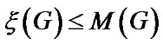 .
.
A contraction of G is obtained by identifying two adjacent vertices of G, and suppressing any loops or multiple edges that arise in this process. A minor of G arises by performing a series of deletions of edges, deletions of isolated vertices, and/or contractions of edges. A graph parameter  is minor monotone if for any minor
  of G,
of G, . The parameter
  was introduced in [6], where it was shown that
  is minor monotone. It was also established that
  and
and  (under the assumptions that
 ) (see [5,7]).
Corollary 2.3 [2,6] Let G be a graph.
1) If  is a minor of G, then

2) If ,
,  and
and  is a minor of G, then

Other possible bounds for minimum rank derived from certain easy to compute parameters of the graph were considered, leading to an investigation of the connection between minimum degree of a vertex,  and minimum rank [8].
Corollary 2.4 For any graph G and infinite field F, 
3. Main Results
In here we calculate the minimum rank of graph . For this purpose we obtained Zero forcing set and the graph parameter
  and the parameter
  and determined the upper bound and lower bound for maximum nullity
 . Since we have
 .
.
Then we can achieve minimum rank of graphs (see Table 1).
Theorem 3.1 For all  and for all graph such that
 , we have
Proof. It is clear that

and 
then

Proposition 3.2 [1] For each of the following families of graphs, :
:
1) Any graph G such that . (The minimum ranks of all graphs of order at most 7 are available in the spreadsheet [9]).
2) 
3) Any tree T.
4) Some families of special graphs.
By this Proposition we have following Theorem.
Theorem 3.3 For each of the following families of graphs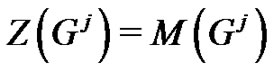 :
:
1) Any graph G such that .
.
2) Complete graph and complete multipartite graph.
3) Petersen graph.
4) Wheel graph.
5) Clebsch Graph for .
.
6) Complement of cycle graph , where
 .
.
Proof. The proof is trivial.
Proposition 3.4 If  be a path graph,
  is homomorphic to the complete graph
 .
.

Table 1. Summary of minimum rank results established in this paper.
Theorem 3.5 For all  we have
Proof. (Figure 1) In graph , we have
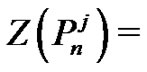
 , because if we start coloring from the end point vertex u, this vertex at least is adjacent with j vertices. The vertex u with its
  adjacent vertices are coloring. The other vertices also are coloring since they are adjacent to coloring vertices, and the number of coloring vertices is j, therefore we have
 . From Corollary 2.2 we have
 .
.
On the other hand with  contraction of the vertices of
 , we reach to the complete graph
 , and we know that
  is a minor for
 . Then we have

Consequently

thus,

(see also [10]).
Proposition 3.6  is homomorphic to
 .
.
Theorem 3.7 , for all
 .
.
Proof. (Figure 2) In  any vertex u is adjacent to 2j vertices, then

On the other hand, . Then

and finally
Proposition 3.8 For all 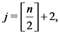 we have
 .
.
Theorem 3.9 For all  we have
 .
.
Proof. (Figures 3, 4, 5) In the jth power of graph  an external vertex
  is adjacent to
  vertices. If we start to coloring of external vertex, then
  vertices are coloring, which
  colored vertices are in external cycle and the remaining vertices are located in the inner cycle. For more coloring we use the nearest adjacent vertex to
  on the set of external vertices. We call this vertex by
 adjacent vertices to
  are same adjacent vertices to
 , and only two of them is different. One of these, which is located on the inner cycle has colored and the another vertex that is located on the external cycle colored from “color-change rule”. We continue the process until all vertices are colored on the internal cycle. Finally

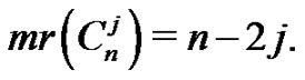
Theorem 3.10 For all  and
and  we have
 .
.
Proof. (Figures 3, 4, 5) when we make  power of
 , then its internal cycle reach to complete graph. With contraction of
  vertices to
  vertices of this graph we reach to complete graph of order
 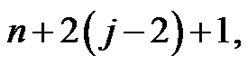 then
then  is a minor of
 . On the other hand we have

Also according to the previous Theorem, we have 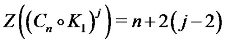 , then

and hence 
Proposition 3.11  is homomorphic to
 .
.
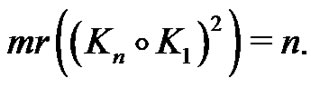
Theorem 3.12 
Proof. (Figures 6, 7) With the contraction of  external vertices of
  on the vertices which is located in internal cycle, we have the complete graph
 , then the minor of
  is
is  So we have

On the other hand it is trivial that . And we have
 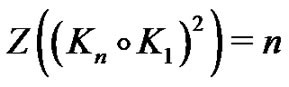 then
then
Proposition 3.13 [1] If G has  vertices and contains a Hamiltonian path, then
 .
.
Theorem 3.14 For all  and
and  vertices we have,
 .
.
Proof. By using the induction on the  it can be shown that
  contains a Hamiltonian path. So we have,
 .
.