Robust Region Tracking for Swarms via a Novel Utilization of Sliding Mode Control ()
1. Introduction
Recently, decentralized control of multiple robotic agents has become an active area of research [1]. Mostly originating from biological inspiration [2-4], the mathematical modeling and control of these “swarms” have advanced to tackle a multitude of problems, such as flocking [5-10], formation flight [11], area coverage [12-15], and even hostile interactions with other swarms [16]. This paper discusses a hybrid procedure for flocking and area coverage.
The specific act of “flocking”, where agents attempt to retain some proximity to their neighbors while aggregateing into a stable formation, has received significant attention. In 2003, Gazi and Passino proposed a first order model [5,6], in which agents were driven to stable flocking behavior by biologically inspired momenta structures. In 2007, Yao et al. extended this concept to a second order model using a sliding mode controller [11]. The controller ensures that the agents’ velocities follow the gradient descent of some desired momenta profiles.
Olfati-Saber handled flocking for a second order model [7] where each agent’s motion is determined by artificial potential energy components. A virtual leader is introduced to prevent fragmentation into smaller groups by creating a common attractive target for all agents. The assumption of universal knowledge of the virtual leader by all the agents is shown to be unnecessary in 2009 by Su et al. [8].
Tanner et al. [9] demonstrates stability of a swarm with no leader for arbitrarily quickly switching network topologies, provided that the swarm remains connected. Zavlanos and Tanner [10] enforce the connectivity of the swarm through a hybrid control. This controller uses local estimates of the network topologies.
Controlled distribution of agents over a wide area (called “coverage control”) is studied by Cortes et al. [12-14]. The majority of these approaches analyze static convex regions. The motion of the agents is determined using gradient descent of some artificial potential.
A hybrid of “flocking” and “area coverage” control of agents inside a moving region is studied in Cheah [15] again using some artificial potential fields. The potential fields are described point wise in the space of the motion, including the inter-agent forces. Our work attempts to solve a similar problem, flocking and area coverage within a target region, but using a completely different approach. We extend the traditional sliding mode controller (SMC) [17] and introduce a new boundary layer concept to achieve the task. This controller competes against modeling uncertainties and bounded unknown forcing functions. The SMC robustly draws all agents towards the target region’s center. However when the agents are inside the region the control is softened allowing the inter-agent repulsive forces to determine the spacing between agents. The region’s perimeter is shown to be upheld successfully by properly selecting the control gains.
Classically, SMC is used for robustizing the control within a desirably small boundary layer [18]. Our novelty lies in performing SMC with a relatively large boundary layer which corresponds to the target region. When the steady state occurs, the swarm will be entrapped within that region. Another critical departure from the traditional SMC is at the deployment of the boundary layer. As described in the text, this leads to a new and desirable feature: sliding occurs at the same time in all spatial dimensions, instead of separate instants.
The resulting decentralized control guides the agents to achieve area coverage within the moving target region. The approach to the target by the agents is asymptotic, and collisions are avoided. Discussions on stability of the controlled dynamics, as well as the disturbance rejection capabilities are included.
The paper is organized as follows: Section 2 covers the governing dynamics of the system and outlines the specific objective. The third section develops the SMC and illustrates its robustness properties for a circular target region. We also provide an analysis of the pessimistic upper bounds for the inter-agent repulsive forces. The effectiveness of such a controller is demonstrated in Section 4. Section 5 expands the analysis to elliptical regions, and the results of this expansion are presented in Section 6. Finally, conclusions are given in Section 7. As a common notation within the text, we denote vectors and matrices with a boldface font, and scalars with italics.
2. System Dynamics and Problem Formulation
In this paper we consider an M-agent swarm in a 2-D environment. Each agent’s dynamics are governed by the following equation
 (1)
(1)
where  is the position vector of the
  agent.
 and
and  are the mass and drag coefficients of that agent. They are assumed to be uncertain modeling parameters with nominal values,
  and
and , and bounded uncertainties,
 (2)
(2)
ui is the control force on the i-th agent and  is the inter-agent repulsion force which is unknown to the controller, except its conservative upperbound
 .
.
These forces are directly linked to the geometric distribution of the agents at any given moment. A focused effort on the formation of these forces and determination of their upperbounds are presented later in the text. The set  contains the positions of neighbors of agent i, defined by
 , where
  is the radius of the neighborhood. We call it the radius of interaction. Only those agents that are in
 , influence the dynamics of agent i. The
  term in (1) represents a friction-like unknown force (indicated by the superscript “u”) which opposes the motion. It is assumed to be smoothly varying and upperbounded,
 .
.
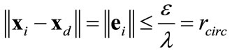
The objective of the control is to drive all agents from a set of arbitrary initial conditions to within a moving circular target region. This region is defined by  , of which
  is the center and
  is the radius. The control should be robust against modeling uncertainties (the mass and the drag constants) as well as the uncertain repulsion and disturbance forces. Initially, we will consider the target region to be a circle, and later the concept will be extended to an ellipse.
Inter-Agent Repulsive Force
The intent of the repulsive forces is to create “personal space” for each agent i, as well as to avoid collision of the agents, by pushing the neighbors away. The resultant of such inter-agent forces on agent i is denoted by . These forces come from those agents within the neighborhood of i and they meet the following criteria:
1) The force is continuous along  and attains its maximum at
 .
.
2) They diminish at the edge of the neighborhood: .
.
In this study, we take the formation of these forces as
 (3)
(3)
They are, however, unknown to the agents except their pessimistic aggregate upperbound. As such, in the control logic they are treated as part of the bounded uncertainty.
3. Sliding Mode Controller (SMC)
The objective of the control is to bring the agents to within the target region, which is taken as a circle for the first part of the paper. Following the traditional SMC formulations [17-19] one starts with the definition of error to be minimized,
 (4)
(4)
which is the vector connecting an individual agent to the center  of the target region. The sliding function is then defined as a Hurwitz combination of the error
 (5)
(5)
The sliding mode controller first reduces  during the “approach phase”, then it maintains
  within a confinement in the pursuant “sliding phase”. In both phases we utilize LaSalle’s theorem [20], to enforce the attracttivity to this confinement. A positive definite Lyapunov candidate for agent i is proposed as
 (6)
(6)
of which the derivative is forced to be negative
 (7)
(7)
Combining (1), (4) and (5), results in
 (8)
(8)
The control,  , is selected such that the
  dynamoics behave according to
 , fulfilling the condition in (7).
The proposed  dynamics, ignoring the uncertainties can be achieved with the deployment of a control as
 (9)
(9)
Substituting (9) into (8), but including the uncertain terms
 (10)
(10)
Considering the worst case contributions of the uncertainties;
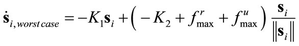 (11)
(11)
Selecting  makes
makes , which forces
  at all times. Notice that
  is a vector. For small
  values, the
  term in the control (9) generally brings undesirable control chatter, i.e., small departures of
  from zero may result in large swings in ui. These swings (chatter) can be alleviated using a saturation function approximation [17-19] within a boundary layer
 (12)
(12)
The treatment up to this point is conventional except the large boundary layer expression . The system’s behavior is robust outside this boundary layer, and the controller (9) is designed to drive the system towards
 . Notice the selection of (12) for
 , at the steady state (i.e.
 ), the error
  remains bounded within
 (13)
(13)
This constitutes the critical departure from the convention and the essence of the novel contribution in this paper.  is not a small boundary width, but large, and it compares to the target region rcirc. Robust controller (9) is softened by the saturation function (12) replacing
 . The objective of this softening is to let the inter-agent repulsion forces,
  , take charge in the distribution of the agents within the target region. Notice that the boundary layer defined in (12) is circular in (s1, s2) space, and so is the respective (x1, x2) counterpart, as per (13). This feature points us to circular target regions most naturally.
In summary, our implementation of the boundary layer is novel and substantially different from the traditional usage. The concept is usurped here to enforce a desired “target state” as opposed to “control chatter abatement”. Thus,  is selected as a finite quantity here, by definition, as opposed to a small number in the conventional deployment, where the size of the boundary layer also influences the control chatter cut-off frequency. We bring a novel philosophy by using the “boundary layer” concept to bound the final distribution of the agents. This provides not only the intended chatter abatement [18,19], but also softens the attraction of the target region’s center. Outside this region, the robustizing term is in full effect and drives the agents towards the region. Inside the region however, it is tolerant towards the inter-agent spacing forces (i.e., repulsion). The control expression in (9) becomes
 (14)
(14)
where the known nominal values of  and
and  are also included. Substituting (14) into (8), the
  -dynamics become
 (15)
(15)
1) When , the dynamics is in the approach phase,
 . The agents are likely to be distant from each other, as per the definition of si given in (5), therefore the repulsive forces are expected to be small. The derivative of the Lyapunov function is
 (16)
(16)
In order to ensure , we select
 (17)
(17)
which guarantees the attractivity of the boundary region .
.
2) When , the agents are more compactly positioned and the
  term grows to be more pronounced. Equations (7) and (15) yield
 (18)
(18)
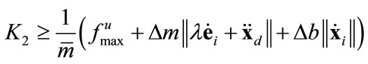
to enforce , at the border of the boundary layer, that is, where
 , we consider the most pessimistic case for uncertainties and select the robustizing gain as
 (19)
(19)
This yields the attractivity of the swarm to within the target circle. Once within the boundary layer, the controlled dynamics would comply with
 (20)
(20)
Equation (20) represents a low pass filter against the perturbation,  (self evident from the previous equation) which entails the uncertainties. This filter attenuates high frequency components of the
  dynamics emanating from perturbations with a cutoff frequency at
 (21)
(21)
This strategy is borrowed from [19], which also contains experimental validation of the concept. Entrapment of the agents within the boundary layer makes the robustizing part of the controller, 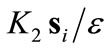 , less effective. Then, the agent distributions are primarily influenced by
 , as well as
  (which is small as velocities are expected to be small). This yields the desired “area capture”.
Notice that (19) suggests a more conservative feedback gain,  , than (17). In order to maintain continuity at the
  boundary, we use (19) throughout.
Evaluation of the Repulsive Force Bound
The upper-bound,  , used in (19) represents the largest resultant force exerted on an agent due to the interagent repulsions and it is assumed known a priori. We present here a numerical procedure to assess that value. When the agents are forced within the target circle, they are expected to space out in a nearly uniform manner. Consequently, those agents at the periphery would be exposed to larger net repulsion forces than those inside. To estimate an extremum for these forces, i.e.,
  , we create a model distribution of uniformly spaced agents within the circular target region. This formation is created by positioning the agents over nested circles with roughly uniform spacing (i.e.,
  in Figure 1 for 30 agents.). We then numerically determine the resultant repulsion forces, using (3), on agents at the periphery (e.g., A in Figure 2) due to agents in the neighborhood (shaded in the figure). Considering isotropic and uniform distribution of agents within a circle, all peripheral agents should be exposed to similar calculated
  values. Target geometries other than a circle would bring anisotropic
  analysis. This point alone confines this scheme to circular targets. We will show the complications even for the elliptical case in latter sections.
4. Case Studies for Circular Targets
In order to demonstrate the effectiveness of the proposed control strategy, we present some case studies. The parameters in Table 1 are common to all cases considered. The circular target is again defined by its center,  , and radius,
 .
.
Case study 1 is on a group of 30 agents aggregating within a non-moving circular region with , using the aforementioned evaluation of
 . The parameters

Figure 1. Model distribution of 30 agents.
 and
and  are fixed but randomly selected based on a uniform probability distribution within the known bounds of uncertainty (
 and
and ). We also consider an unknown, time-varying friction-like force,
  which is only known to the controller by its upperbound
 .
.
Figure 3 shows the time-lapsed frames of the dynamoics. The agents inside the region remain almost evenly distributed, which indicates that our prediction of supremum of repulsion forces,  , is appropriate. The first two frames do not have as many agents due to their selected remote starting positions.
We introduce a numerical metric for a quantitative comparison among various agent distributions vis-à-vis the target region to be occupied. It is called the coverage index and defined by:
 (22)
(22)
where  is the average of the minimum distances of each agent
 (23)
(23)
ri, min is the distance of agent i to its nearest neighbor; A is the area of the target region, and M is the number of agents. This dimensionless quantity, C, is close to 1 for a uniformly spaced distribution within the target region. C
> 1 and C < 1 would imply dispersion outside the target region and bunching up within the target region cases respectively.
The variation of C in time is shown in Figure 4 for this case study. The values marked correspond to the 4, 6 and 8 sec. snapshots depicted in Figure 3. The measure, C, of coverage fully describes the slightly bunched coverage in the last frame (i.e., 8 sec.),  simply indicates that the determination of
  was over conservative.
Case study 2 (Figure 5) shows 60 agents tracking a moving circular region of radius 2, the center of which is moving according to  which is shown as a trace in Figure 5. All of the agents again aggregate inside the region despite the parameter uncertainties, upper-bounded unknown forces, and inter-agent repulsion forces.
Following the quantitative discussion on Case study 1 we present the coverage index variations for this example (see Figure 6). Again, the corresponding points of 4, 5, 6 and 10 sec. snapshots in Figure 5 are displayed in this figure.
One can notice that  declares a uniform and desirable filling of the circular target at 10 sec. This is achieved despite the uncertainties in the dynamics and moving target region, which shows a very effective control.
Time traces of  are shown in Figure 7. The agent enters the sliding phase within 0.8 seconds, which roughly corresponds to 4 times the time constant
  seconds of (15) starting from large values of
 . Note the sliding manifold of
 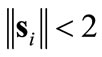 is unnoticeably small in the figure.
Figure 8 shows the control force, repulsive forces and the uncertain force on the same agent. The resultant of all forces on the agent at the steady state is periodic in nature, corresponding to the motion of the moving region.