A Rational Approximation of the Fourier Transform by Integration with Exponential Decay Multiplier

Sanjar M. Abrarov^1,2, Rehan Siddiqui^2,3,4, Rajinder K. Jagpal^3,4, Brendan M. Quine^1,2,4

¹Thoth Technology Inc., Algonquin Radio Observatory, Pembroke, ON, Canada.
²Department of Earth and Space Science and Engineering, York University, Toronto, Canada.
³Epic College of Technology, Mississauga, Canada.
⁴Department of Physics and Astronomy, York University, Toronto, Canada.

DOI: 10.4236/am.2021.1211063                

Abstract

Recently we have reported a new method of rational approximation of the sinc function obtained by sampling and the Fourier transforms. However, this method requires a trigonometric multiplier that originates from the shifting property of the Fourier transform. In this work, we show how to represent the Fourier transform of a function f(t) in form of a ratio of two polynomials without any trigonometric multiplier. A MATLAB code showing algorithmic implementation of the proposed method for rational approximation of the Fourier transform is presented.

Keywords

Rational Approximation, Fourier Transform, Sampling, Sinc Function

1. Introduction

The forward and inverse Fourier transforms of two related functions $f\left(t\right)$ and $F\left(\nu \right)$ can be defined in a symmetric form as [1] [2]:

$\mathcal{F}\left\{f\left(t\right)\right\}\left(\nu \right)=F\left(\nu \right)={\displaystyle \underset{-\infty }{\overset{\infty }{\int }}}f\left(t\right){\text{e}}^{-2\pi i\nu t}\text{d}t$ (1)

and:

${\mathcal{F}}^{-1}\left\{F\left(\nu \right)\right\}\left(t\right)=f\left(t\right)={\displaystyle \underset{-\infty }{\overset{\infty }{\int }}}F\left(\nu \right){\text{e}}^{2\pi i\nu t}\text{d}\nu ,$ (2)

where variables t and $\nu$ are the corresponding Fourier-transformed arguments in t-space and $\nu$ -space, respectively (time t vs. frequency $\nu$, for example).

Fourier transform methods are widely used in many applications including signal processing [1] [2], spectroscopy [3] [4] and computational finance [5] [6] [7].

There are several efficient methods that have been reported for rational approximations in literature. For example, the rational approximations may be built on the basis of the Newman nodes [8], Chebyshev nodes [9], logarithmic nodes [10] and so on.

Recently we have reported a new method of rational approximation of the Fourier transform (1) as given by [11]:

$\mathcal{F}\left\{f\left(t\right)\right\}\left(\nu \right)\approx {\text{e}}^{2\pi i\nu a}{\displaystyle \underset{m=1}{\overset{2^{M-1}}{\sum }}}\frac{A_m\left(\sigma +2\pi i\nu \right)+B_m}{C_m^2+{\left(\sigma +2\pi i\nu \right)}^2}\mathrm{,}$ (3)

where M is an integer determining the number of summation terms $2^{M-1}$, $a$ is a shift constant, $\sigma$ is a decay (damping) constant and:

$A_m=\frac{1}{2^{M-1}}{\displaystyle \underset{n=0}{\overset{N}{\sum }}}f\left(nh-a\right){\text{e}}^{\sigma nh}\cos \left(C_{m}nh\right),$

$B_m=\frac{1}{2^{M-1}}{\displaystyle \underset{n=0}{\overset{N}{\sum }}}f\left(nh-a\right){\text{e}}^{\sigma nh}{C}_m\sin \left(C_{m}nh\right),$

$C_m=\frac{\pi \left(2m-1\right)}{2^{M}h}.$

are expansion coefficients.

It has been noticed that approximation (3) is not purely rational and there was a question whether or not a rational function of the Fourier transform (1) in explicit form without any trigonometric multiplier of the kind:

${\text{e}}^{2\pi i\nu a}=\cos \left(2\pi \nu a\right)+i\sin \left(2\pi \nu a\right),$ (4)

depending on the argument $\nu$, can be obtained [12]. Theoretical analysis shows that this trigonometric multiplier originating from the shifting property of the Fourier transform can be indeed excluded. As a further development of our work [11], in this paper, we derive a rational function of the Fourier transform (1) that has no any trigonometric multiplier of the kind (4). Therefore, it can be used as an alternative to the Padé approximation. To the best of our knowledge, this method of rational approximation of the Fourier transform (1) for a non-periodic function $f\left(t\right)$ has never been reported in scientific literature.

2. Derivation

2.1. Preliminaries

Assume that $\mathrm{Re}\left\{f\left(t\right)\right\}$ is even while $\mathrm{Im}\left\{f\left(t\right)\right\}$ is odd such that $f\mathrm{<mo>\; :\; </mo>}ℝ\to ℂ$, but $\mathrm{Re}\left\{f\right\}:ℝ\to ℝ$ and $\mathrm{Im}\left\{f\right\}:ℝ\to ℝ$. Then it is not difficult to see that the Fourier transform (1) of the function $f\left(t\right)$ can be expanded into two integral terms as follows:

$\mathcal{F}\left\{f\left(t\right)\right\}\left(\nu \right)=F\left(\nu \right)=2{\displaystyle \underset{0}{\overset{\infty }{\int }}}\mathrm{Re}\left\{f\left(t\right)\right\}\cos \left(2\pi \nu t\right)\text{d}t+2{\displaystyle \underset{0}{\overset{\infty }{\int }}}\mathrm{Im}\left\{f\left(t\right)\right\}\sin \left(2\pi \nu t\right)\text{d}t.$

Assume also that the function $f\left(t\right)$ behaves in such a way that for some positive numbers ${\tau }_1$ and ${\tau }_2$ the following integrals:

${\displaystyle \underset{{\tau }_1}{\overset{\infty }{\int }}}\mathrm{Re}\left\{f\left(t\right)\right\}\cos \left(2\pi \nu t\right)\text{d}t\approx 0$

and:

${\displaystyle \underset{{\tau }_2}{\overset{\infty }{\int }}}\mathrm{Im}\left\{f\left(t\right)\right\}\sin \left(2\pi \nu t\right)\text{d}t\approx 0$

are negligibly small and can be ignored in computation. Consequently, we can approximate the Fourier transform as given by:

$\mathcal{F}\left\{f\left(t\right)\right\}\left(\nu \right)=F\left(\nu \right)\approx 2{\displaystyle \underset{0}{\overset{{\tau }_1}{\int }}}\mathrm{Re}\left\{f\left(t\right)\right\}\cos \left(2\pi \nu t\right)\text{d}t+2{\displaystyle \underset{0}{\overset{{\tau }_2}{\int }}}\mathrm{Im}\left\{f\left(t\right)\right\}\sin \left(2\pi \nu t\right)\text{d}t.$ (5)

Further the values $2{\tau }_1$ and $2{\tau }_2$ will be regarded as widths (pulse widths) for the real and imaginary parts of the function $f\left(t\right)$, respectively.

2.2. New Sampling Method

Consider a sampling Formula (see, for example, Equation (3) in [13] ):

$f\left(t\right)={\displaystyle \underset{n=-N}{\overset{N}{\sum }}}f\left(t_n\right)\text{sinc}\left(\frac{\pi }{h}\left(t-t_n\right)\right)+\epsilon \left(t\right),$ (6)

where:

$\text{sinc}\left(t\right)=\{\begin{array}{l}\frac{\sin t}{t}\mathrm{,}t\ne 0\\ \mathrm{1,}t=\mathrm{0,}\end{array}$

is the sinc function, $t_n$ is a set of sampling points, h is small adjustable parameter (step) and $\epsilon \left(t\right)$ is error term. François Viète discovered that the sinc function can be represented by cosine product¹ [14] [15]:

$\text{sinc}\left(t\right)={\displaystyle \underset{m=1}{\overset{\infty }{\prod }}}\cos \left(\frac{t}{2^m}\right)\mathrm{.}$ (7)

In our earlier publications we introduced a product-to-sum identity [16]:

${\displaystyle \underset{m=1}{\overset{M}{\prod }}}\cos \left(\frac{t}{2^m}\right)=\frac{1}{2^{M-1}}{\displaystyle \underset{m=1}{\overset{2^{M-1}}{\sum }}}\cos \left(\frac{2m-1}{2^M}t\right)$ (8)

and applied it for sampling [17] [18] as incomplete cosine expansion of the sinc function for efficient computation of the Voigt/complex error function. It is worth noting that this product-to-sum identity has also found some efficient applications in computational finance [6] [19] [20] involving numerical integration.

Comparing identities (7) and (8) immediately yields:

$\text{sinc}\left(t\right)=\underset{M\to \infty }{lim}\frac{1}{2^{M-1}}{\displaystyle \underset{m=1}{\overset{2^{M-1}}{\sum }}}\cos \left(\frac{m-1/2}{2^{M-1}}t\right)\mathrm{.}$

Unlike Equation (7), this limit consists of sum of cosines instead of product of cosines. As a result, its application provides significant flexibilities in various numerical integrations [6] [17] [18] [19] [20].

Change of variable $2^{M-1}\to M$ in the limit above leads to:

$\text{sinc}\left(t\right)=\underset{M\to \infty }{lim}\frac{1}{M}{\displaystyle \underset{m=1}{\overset{M}{\sum }}}\cos \left(\frac{m-1/2}{M}t\right)\mathrm{.}$

Therefore, by truncating integer M and by making another change of variable $t\to \pi t/h$ we obtain:

$\text{sinc}\left(\frac{\pi }{h}t\right)\approx \frac{1}{M}{\displaystyle \underset{m=1}{\overset{M}{\sum }}}\cos \left(\frac{\pi \left(m-1/2\right)}{Mh}t\right)\mathrm{,}-Mh\le t\le Mh\mathrm{.}$ (9)

The right side of Equation (9) is periodic due to finite number of the summation terms. As a result, the approximation (9) is valid only within the interval $t\in \left[-Mh\mathrm{,}Mh\right]$.

At equidistantly separated sampling grid-points such that $t_n=nh$, the substitution of approximation (9) into sampling Formula (6) gives:

$f\left(t\right)\approx \frac{1}{M}{\displaystyle \underset{m=1}{\overset{M}{\sum }}}{\displaystyle \underset{n=-N}{\overset{N}{\sum }}}f\left(nh\right)\cos \left(\frac{\pi \left(m-1/2\right)}{Mh}\left(t-nh\right)\right)\mathrm{,}-Mh\le t\le Mh\mathrm{.}$ (10)

It is important that in sampling procedure the total number of the sampling grid-points $2N+1$ as well as the step h should be properly chosen to insure that the widths $2{\tau }_1$ and $2{\tau }_2$ are entirely covered.

As we can see, the sampling Formula (10) is based on incomplete cosine expansion of the sinc function that was proposed in our previous works [17] [18] as a new approach for rapid and highly accurate computation of the Voigt/complex error function [21] [22] [23]. Computations we performed show that this method of sampling is particularly efficient in numerical integration.

2.3. Even Function

Suppose that our objective is to approximate the sinc function $\text{sinc}\left(\pi \nu \right)$. First we take the inverse Fourier transform (2) of the sinc function:

${\mathcal{F}}^{-1}\left\{\text{sinc}\left(\pi \nu \right)\right\}\left(t\right)={\displaystyle \underset{-\infty }{\overset{\infty }{\int }}}\text{sinc}\left(\pi \nu \right){\text{e}}^{-2\pi i\nu t}\text{d}\nu =\text{rect}\left(t\right)\mathrm{,}$

where:

$\text{rect}\left(t\right)=\{\begin{array}{l}\mathrm{1,}\text{if}\left|t\right|<1/2\\ 1/2\mathrm{,}\text{if}\left|t\right|=1/2\\ \mathrm{0,}\text{if}\left|t\right|>1/2\mathrm{,}\end{array}$

is known as the rectangular function. This function is even since $\text{rect}\left(t\right)=\text{rect}\left(-t\right)$. The rectangular function $\text{rect}\left(t\right)$ has two discontinuities at $t=-1/2$ and $t=1/2$. Therefore, it is somehow problematic to perform sampling over this function. However, we can use the fact that:

$\text{rect}\left(t\right)=\underset{k\to \infty }{lim}\frac{1}{{\left(2t\right)}^{2k}+1}\mathrm{.}$ (11)

Thus, by taking a sufficiently large value for the integer k, say $k=35$, we can approximate the rectangular function (11) quite accurately as:

$\text{rect}\left(t\right)\approx f\left(t\right)=\frac{1}{{\left(2t\right)}^{70}+1}\mathrm{.}$

Figure 1 shows the function $f\left(t\right)=1/\left({\left(2t\right)}^{70}+1\right)$ by blue curve. As we can see from this figure, the function very rapidly decreases at $\left|t\right|>1/2$ with increasing t. Therefore, we can take ${\tau }_1=0.6$. Thus, the width of this function is $2{\tau }_1=1.2$.

Sampling of function $f\left(t\right)=1/\left({\left(2t\right)}^{70}+1\right)$ in accordance with Equation (10) results in a periodic dependence. Consequently, due to periodicity on the right side of Equation (10) it cannot be utilized for rational approximation of the Fourier transform. However, this problem can be effectively resolved by sampling the function $f\left(t\right){\text{e}}^{\sigma t}$ instead of $f\left(t\right)$ itself. This leads to:

$f\left(t\right){\text{e}}^{\sigma t}\approx \frac{1}{M}{\displaystyle \underset{m=1}{\overset{M}{\sum }}}{\displaystyle \underset{n=-N}{\overset{N}{\sum }}}f\left(nh\right){\text{e}}^{\sigma nh}\cos \left(\frac{\pi \left(m-1/2\right)}{Mh}\left(t-nh\right)\right)\mathrm{,}-Mh\le t\le Mh\mathrm{.}$ (12)

Figure 2 shows the results of computation for even function $f\left(t\right)=1/\left({\left(2t\right)}^{70}+1\right)$ by approximation (12) at $M=32$, $N=28$, $h=0.04$ with $\sigma =0$ (blue curve), $\sigma =0.25$ (red curve) and $\sigma =0.75$ (green curve). As we can see from this figure, all three curves are periodic as expected. However, if the constant $\sigma$ is big enough, then slight rearrangement of Equation (12) in form:

$f\left(t\right)\approx \frac{{\text{e}}^{-\sigma t}}{M}{\displaystyle \underset{m=1}{\overset{M}{\sum }}}{\displaystyle \underset{n=-N}{\overset{N}{\sum }}}f\left(nh\right){\text{e}}^{\sigma nh}\cos \left(\frac{\pi \left(m-1/2\right)}{Mh}\left(t-nh\right)\right)\mathrm{,}$ (13)

can effectively eliminate this periodicity due to presence of the exponential decay multiplier ${\text{e}}^{-\sigma t}$ on the right side. This suppression effect can be seen from

Figure 1. The even $1/\left({\left(2t\right)}^{70}+1\right)$ and odd $t/\left({\left(2t\right)}^{70}+1\right)$ functions shown by blue and red curves, respectively.

Figure 2. Approximation (12) to the function $f\left(t\right){\text{e}}^{\sigma t}={\text{e}}^{\sigma t}/\left[{\left(2t\right)}^{70}+1\right]$ computed at $M=32$, $N=28$, $h=0.04$ with $\sigma =0$ (blue curve), $\sigma =0.25$ (red curve) and $\sigma =0.75$ (green curve).

Figure 3 illustrating the results of computation for the even function $f\left(t\right)=1/\left({\left(2t\right)}^{70}+1\right)$ by approximation (13) at $M=32$, $N=28$ with $\sigma =0$ (blue curve), $\sigma =0.25$ (red curve) and $\sigma =0.75$ (green curve). As it is depicted by blue curve, at $\sigma =0$ the function is periodic. However, as decay coefficient $\sigma$ increases, the exponential multiplier ${\text{e}}^{-\sigma t}$ suppresses all the peaks (except the first peak at the origin) such that the resultant function tends to become solitary along the entire positive t-axis. This tendency can be observed by red and green curves at $\sigma =0.25$ and $\sigma =0.75$, respectively. As a consequence, if the damping multiplier $\sigma$ is big enough, say greater than unity, the approximated function becomes practically solitary as the original function $f\left(t\right)=1/\left({\left(2t\right)}^{70}+1\right)$ itself.

Thus, substituting approximation (13) into Equation (5) and considering the fact that at sufficiently large $\sigma$ the function becomes solitary along positive x-axis, the upper limit ${\tau }_1$ of integration can be replaced by infinity as²:

$\begin{array}{l}\mathcal{F}\left\{f\left(t\right)\right\}\left(\nu \right)=\mathcal{F}\left\{\mathrm{Re}\left\{f\left(t\right)\right\}\right\}\left(\nu \right)=\mathcal{F}\left\{\frac{1}{{\left(2t\right)}^{70}+1}\right\}\left(\nu \right)\\ \approx 2{\displaystyle \underset{0}{\overset{{\tau }_1}{\int }}}\left[\frac{{\text{e}}^{-\sigma t}}{M}{\displaystyle \underset{m=1}{\overset{M}{\sum }}}{\displaystyle \underset{n=-N}{\overset{N}{\sum }}}\mathrm{Re}\left\{f\left(nh\right)\right\}{\text{e}}^{\sigma nh}\cos \left(\frac{\pi \left(m-1/2\right)}{Mh}\left(t-nh\right)\right)\right]\cos \left(2\pi \nu t\right)\text{d}t\\ \approx 2{\displaystyle \underset{0}{\overset{\infty }{\int }}}\left[\frac{{\text{e}}^{-\sigma t}}{M}{\displaystyle \underset{m=1}{\overset{M}{\sum }}}{\displaystyle \underset{n=-N}{\overset{N}{\sum }}}\mathrm{Re}\left\{f\left(nh\right)\right\}{\text{e}}^{\sigma nh}\cos \left(\frac{\pi \left(m-1/2\right)}{Mh}\left(t-nh\right)\right)\right]\cos \left(2\pi \nu t\right)\text{d}t.\end{array}$

This integral can be taken analytically in form of rational function now and after some trivial rearrangements that exclude double summation, it follows that

$\mathcal{F}\left\{\mathrm{Re}\left\{f\left(t\right)\right\}\right\}\left(\nu \right)\approx {\displaystyle \underset{m=1}{\overset{M}{\sum }}}\frac{{\alpha }_m+{\beta }_m{\nu }^2}{{\kappa }_m+{\lambda }_m{\nu }^2+{\nu }^4},$ (14)

where the expansion coefficients are given by:

Figure 3. Evolution to the function $f\left(t\right)=1/\left[{\left(2t\right)}^{70}+1\right]$ computed by approximation (13) at $M=32$, $N=28$, $h=0.04$ with $\sigma =0$ (blue curve), $\sigma =0.25$ (red curve) and $\sigma =0.75$ (green curve).

${\alpha }_m=\frac{1}{8M{\pi }^4}{\displaystyle \underset{n=-N}{\overset{N}{\sum }}}\mathrm{Re}\left\{f\left(nh\right)\right\}{\text{e}}^{nh\sigma }\left({\mu }_m^2+{\sigma }^2\right)\left(\sigma \cos \left(nh{\mu }_m\right)+{\mu }_m\sin \left(nh{\mu }_m\right)\right),$

${\beta }_m=\frac{1}{2M{\pi }^2}{\displaystyle \underset{n=-N}{\overset{N}{\sum }}}\mathrm{Re}\left\{f\left(nh\right)\right\}{\text{e}}^{nh\sigma }\left(\sigma \cos \left(nh{\mu }_m\right)-{\mu }_m\sin \left(nh{\mu }_m\right)\right),$

${\kappa }_m=\frac{1}{16{\pi }^4}{\left({\mu }_m^2+{\sigma }^2\right)}^2,$

${\lambda }_m=\frac{1}{2{\pi }^2}\left({\sigma }^2-{\mu }_m^2\right)$

and:

${\mu }_m=\frac{\pi \left(m-1/2\right)}{Mh}\mathrm{.}$

Figure 4 shows the original sinc function $\text{sinc}\left(\nu \right)$ and its approximation (14) within the interval $-2\pi \le \nu \le 2\pi$ at $M=32$, $N=28$, $h=0.04$ and $\sigma =2.75$ by black dashed and light blue curves, respectively. These two curves are not visually distinctive.

2.4. Odd Function

Consider, as an example, the following function:

$f\left(t\right)=\frac{it}{{\left(2t\right)}^{70}+1}\approx it\text{rect}\left(t\right)\mathrm{.}$

We can see that the condition $t\text{r}ect\left(t\right)=-\left(-t\text{r}ect\left(-t\right)\right)$ for odd function in its imaginary part is satisfied. The function $\mathrm{Im}\left\{f\left(t\right)\right\}=t/\left({\left(2t\right)}^{70}+1\right)$ is shown in Figure 1 by red curve. We can take ${\tau }_2=0.6$ and the width is $2{\tau }_2=1.2$.

Using exactly same procedure as it has been described above and considering the fact that at sufficiently large $\sigma$ the upper limit ${\tau }_2$ of integration can be replaced by infinity, we can write³:

Figure 4. Approximations of the functions $\text{sinc}\left(\pi \nu \right)$ and $\left(\sin \left(\pi \nu \right)-\pi \nu \cos \left(\pi \nu \right)\right)/\left(2{\left(\pi \nu \right)}^2\right)$ within interval $-2\pi \le \nu \le 2\pi$. Both approximations are obtained by Equations (14), (15) for input functions $1/\left({\left(2t\right)}^{70}+1\right)$ and $it/\left({\left(2t\right)}^{70}+1\right)$ at $M=32$, $N=28$, $h=0.04$, $\sigma =2.7$ (light blue curve) and at $M=32$, $N=28$, $h=0.04$, $\sigma =3$ (gray curve), respectively. The original functions $\text{sinc}\left(\pi \nu \right)$ and $\left(\sin \left(\pi \nu \right)-\pi \nu \cos \left(\pi \nu \right)\right)/\left(2{\left(\pi \nu \right)}^2\right)$ are also shown by black dashed curves for comparison.

$\begin{array}{l}\mathcal{F}\left\{f\left(t\right)\right\}\left(\nu \right)=\mathcal{F}\left\{i\mathrm{Im}\left\{f\left(t\right)\right\}\right\}\left(\nu \right)=\mathcal{F}\left\{i\frac{t}{{\left(2t\right)}^{70}+1}\right\}\left(\nu \right)\\ \approx 2{\displaystyle \underset{0}{\overset{{\tau }_2}{\int }}}\left[\frac{{\text{e}}^{-\sigma t}}{M}{\displaystyle \underset{m=1}{\overset{M}{\sum }}}{\displaystyle \underset{n=-N}{\overset{N}{\sum }}}\mathrm{Im}\left\{f\left(nh\right)\right\}{\text{e}}^{\sigma nh}\cos \left(\frac{\pi \left(m-1/2\right)}{Mh}\left(t-nh\right)\right)\right]\sin \left(2\pi \nu t\right)\text{d}t\\ \approx 2{\displaystyle \underset{0}{\overset{\infty }{\int }}}\left[\frac{{\text{e}}^{-\sigma t}}{M}{\displaystyle \underset{m=1}{\overset{M}{\sum }}}{\displaystyle \underset{n=-N}{\overset{N}{\sum }}}\mathrm{Im}\left\{f\left(nh\right)\right\}{\text{e}}^{\sigma nh}\cos \left(\frac{\pi \left(m-1/2\right)}{Mh}\left(t-nh\right)\right)\right]\sin \left(2\pi \nu t\right)\text{d}t.\end{array}$

This leads to:

$\mathcal{F}\left\{i\mathrm{Im}\left\{f\left(t\right)\right\}\right\}\left(\nu \right)\approx {\displaystyle \underset{m=1}{\overset{M}{\sum }}}\frac{{\eta }_m\nu +{\theta }_m{\nu }^3}{{\kappa }_m+{\lambda }_m{\nu }^2+{\nu }^4},$ (15)

where the expansion coefficients are:

${\eta }_m=\frac{1}{4M{\pi }^3}{\displaystyle \underset{n=-N}{\overset{N}{\sum }}}\mathrm{Im}\left\{f\left(nh\right)\right\}{\text{e}}^{nh\sigma }\left(\left({\sigma }^2-{\mu }_m^2\right)\cos \left(nh{\mu }_m\right)+2\sigma {\mu }_m\sin \left(nh{\mu }_m\right)\right)$

and:

${\theta }_m=\frac{1}{M\pi }{\displaystyle \underset{n=-N}{\overset{N}{\sum }}}\mathrm{Im}\left\{f\left(nh\right)\right\}{\text{e}}^{nh\sigma }\cos \left(nh{\mu }_m\right).$

The Fourier transform of the function $it\text{rect}\left(t\right)$ can be readily found analytically:

$\begin{array}{c}\mathcal{F}\left\{it\text{rect}\left(t\right)\right\}\left(\nu \right)={\displaystyle \underset{-\infty }{\overset{\infty }{\int }}}it\text{rect}\left(t\right){\text{e}}^{-2\pi i\nu t}\text{d}t={\displaystyle \underset{-1/2}{\overset{1/2}{\int }}}it\text{rect}\left(t\right){\text{e}}^{-2\pi i\nu t}\text{d}t\\ ={\displaystyle \underset{-1/2}{\overset{1/2}{\int }}}it{\text{e}}^{-2\pi i\nu t}\text{d}t=\frac{\sin \left(\pi \nu \right)-\pi \nu \cos \left(\pi \nu \right)}{2{\left(\pi \nu \right)}^2}\mathrm{.}\end{array}$

Gray curve in Figure 4 illustrates the Fourier transform of the function $f\left(t\right)=it/\left({\left(2t\right)}^{70}+1\right)$ obtained by using approximation (15) at $M=32$, $N=28$, $h=0.04$ and $\sigma =3$. The original function:

$\mathcal{F}\left\{it\text{rect}\left(t\right)\right\}\left(\nu \right)=\frac{\sin \left(\pi \nu \right)-\pi \nu \cos \left(\pi \nu \right)}{2{\left(\pi \nu \right)}^2}$

is also shown for comparison by black dashed curve. These two curves in the interval $-2\pi \le \nu \le 2\pi$ are also not distinctive visually.

3. Accuracy

Figure 5 shows the absolute difference between original sinc function $\text{sinc}\left(\pi \nu \right)$ and its approximation (14) for input function $f\left(t\right)=1/\left({\left(2t\right)}^{70}+1\right)$ calculated at $M=32$, $N=28$, $h=0.04$ and $\sigma =2.7$. As we can see, the absolute difference within the interval $-2\pi \le \nu \le 2\pi$ does not exceed 2.5 × 10⁻³. This accuracy is better than that of shown in our recent publication, where we used Equation (3) for the sinc function approximation (see Figure 6 in [11] ).

Figure 6 shows the absolute difference between original function given by $\left(\sin \left(\pi \nu \right)-\pi \nu \cos \left(\pi \nu \right)\right)/\left(2{\left(\pi \nu \right)}^2\right)$ and its approximation (15) for input function $f\left(t\right)=it/\left({\left(2t\right)}^{70}+1\right)$ calculated at $M=32$, $N=28$, $h=0.04$ and $\sigma =3$. We can see that the absolute difference within the interval $-2\pi \le \nu \le 2\pi$ does not exceed 6 × 10⁻⁴.

It should be noted that with more well-behaved functions we can obtain considerably higher accuracies. For example, suppose that we need to obtain the Fourier transform of the function $f\left(t\right)=\sqrt{\pi }{\text{e}}^{-{\left(\pi t\right)}^2}+i\left[{\pi }^{3/2}t{\text{e}}^{-{\left(\pi t\right)}^2}\right]$ by using approximations (14) and (15). Analytically, its Fourier transform is:

$\mathcal{F}\left\{\sqrt{\pi }{\text{e}}^{-{\left(\pi t\right)}^2}+i\left[{\pi }^{3/2}t{\text{e}}^{-{\left(\pi t\right)}^2}\right]\right\}\left(\nu \right)={\text{e}}^{-{\nu }^2}+\nu {\text{e}}^{-{\nu }^2}\mathrm{,}$

Figure 5. Absolute difference between the original sinc function $\text{sinc}\left(\pi \nu \right)$ and its rational approximation (14) for input function $f\left(t\right)=1/\left({\left(2t\right)}^{70}+1\right)$ at $M=32$, $N=28$, $h=0.04$ and $\sigma =2.7$.

Figure 6. Absolute difference between the original function $\left(\sin \left(\pi \nu \right)-\pi \nu \cos \left(\pi \nu \right)\right)/\left(2{\left(\pi \nu \right)}^2\right)$ and its rational approximation (15) for input function $f\left(t\right)=it/\left({\left(2t\right)}^{70}+1\right)$ at $M=32$, $N=28$, $h=0.04$ and $\sigma =3$.

where ${\text{e}}^{-{\nu }^2}$ is the Fourier transform of $\sqrt{\pi }{\text{e}}^{-{\left(\pi t\right)}^2}$ while $\nu {\text{e}}^{-{\nu }^2}$ is the Fourier transform of $i{\pi }^{3/2}t{\text{e}}^{-{\left(\pi t\right)}^2}$.

Blue curve in Figure 7 corresponds to the absolute difference between function ${\text{e}}^{-{\nu }^2}$ and its approximation (14) for input function $\sqrt{\pi }{\text{e}}^{-{\left(\pi t\right)}^2}$ at $M=16$, $N=23$, $h=0.119$ and $\sigma =6.9$. Red curve in Figure 7 corresponds to the absolute difference between function $\nu {\text{e}}^{-{\nu }^2}$ and its approximation (15) for input function $i{\pi }^{3/2}t{\text{e}}^{-{\left(\pi t\right)}^2}$ at $M=16$, $N=23$, $h=0.119$ and $\sigma =5.9$. We can see that with only 16 summation terms the absolute differences do not exceed 3 × 10⁻¹⁰ and 9 × 10⁻¹⁰. These results demonstrate that the rational approximations (14) and (15) can be highly accurate in the Fourier transform of well-behaved functions.

In our recent work [24] we applied alternative method of sampling by using incomplete cosine expansion of the Gaussian function of kind $h{\text{e}}^{-{\left(t/c\right)}^2}/\left(c\sqrt{\pi }\right)$, where c and h are the fitting parameters. We have shown that this method of sampling can also be used to obtain high-accuracy computation of the Voigt/complex error function. In our future work will apply this method of sampling as an alternative that may reduce the absolute difference for rational approximations of the piecewise functions with discontinuities.

4. Alternative Representation

For a function $f\left(t\right)=\mathrm{Re}\left\{f\left(t\right)\right\}+i\mathrm{Im}\left\{f\left(t\right)\right\}$, where its real part $\mathrm{Re}\left\{f\left(t\right)\right\}$ is even and its imaginary part $\mathrm{Im}\left\{f\left(t\right)\right\}$ is odd, we can write:

$\mathcal{F}\left\{f\left(t\right)\right\}\left(\nu \right)\approx {\displaystyle \underset{m=1}{\overset{M}{\sum }}}\frac{{\alpha }_m+{\beta }_m{\nu }^2}{{\kappa }_m+{\lambda }_m{\nu }^2+{\nu }^4}+{\displaystyle \underset{m=1}{\overset{M}{\sum }}}\frac{{\eta }_m\nu +{\theta }_m{\nu }^3}{{\kappa }_m+{\lambda }_m{\nu }^2+{\nu }^4}$

or:

$\mathcal{F}\left\{f\left(t\right)\right\}\left(\nu \right)\approx {\displaystyle \underset{m=1}{\overset{M}{\sum }}}\frac{{\alpha }_m+{\eta }_m\nu +{\beta }_m{\nu }^2+{\theta }_m{\nu }^3}{{\kappa }_m+{\lambda }_m{\nu }^2+{\nu }^4}.$

Figure 7. Absolute difference between the original functions ${\text{e}}^{-{\nu }^2}$ and its approximation (14) for input function $\sqrt{\pi }{\text{e}}^{-{\left(\pi t\right)}^2}$ at $M=16$, $N=23$, $h=0.04$ and $\sigma =6.9$ (blue curve). Absolute difference between the original functions $\nu {\text{e}}^{-{\nu }^2}$ and its approximation (15) for input function $i{\pi }^{3/2}t{\text{e}}^{-{\left(\pi t\right)}^2}$ at $M=16$, $N=23$, $h=0.04$ and $\sigma =5.9$ (red curve).

Using a Computer Algebra System (CAS) supporting symbolic programming it is not difficult to find coefficients $p_k$ and $q_k$ to represent this approximation as:

$\mathcal{F}\left\{f\left(t\right)\right\}\left(\nu \right)\approx \frac{P\left(\nu \right)}{Q\left(\nu \right)}\mathrm{,}$ (16)

where:

$P\left(\nu \right)=p_0+p_1\nu +p_2{\nu }^2+\cdots +p_{4M-2}{\nu }^{4M-2}+p_{4M-1}{\nu }^{4M-1}$

and:

$Q\left(\nu \right)=q_0+q_1{\nu }^2+q_2{\nu }^4+\cdots +q_{2M-1}{\nu }^{4M-2}+q_{2M}{\nu }^{4M},$

are polynomials of the orders $4M-1$ and $4M$, respectively.

Padé approximation is one of the efficient methods to represent a function in form of ratio of two polynomials. Our preliminary numerical results show that the proposed new method of rational approximation may significantly extend the range $\left[{\nu }_{\min },{\nu }_{\max }\right]$ in coverage [12] than the conventional Padé approximation.

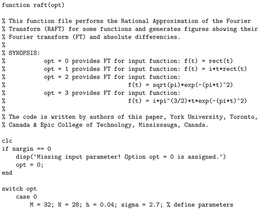
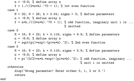
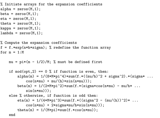
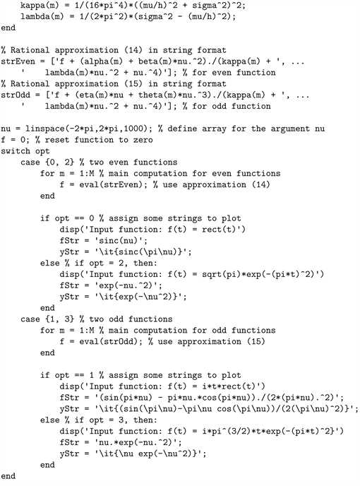
5. MATLAB Code and Description

The MATLAB code shown below is written as a function file raft.m that can be simply copied and pasted to create m-file in the MATLAB environment. The name of this function file originates from the abbreviation RAFT that stands for Rational Approximation of the Fourier transform. The command raft(opt) performs sampling and then computation of the expansion coefficients ${\alpha }_m$, ${\beta }_m$, ${\eta }_m$, ${\theta }_m$, ${\kappa }_m$, ${\lambda }_m$, ${\mu }_m$. Once the coefficients are determined, the program executes the Fourier transform according to Equations (14) and (15) for even and odd input functions, respectively. The results of computations are generated in two plots. The first plot shows the Fourier transform of input function while the second plot illustrates its absolute difference.

There are four option values for opt argument. At opt = 0, opt = 1, opt = 2 and opt = 3 the corresponding input functions are $\text{rect}\left(t\right)$, $it\text{rect}\left(t\right)$, $\sqrt{\pi }{\text{e}}^{-{\left(\pi t\right)}^2}$ and $i{\pi }^{3/2}t{\text{e}}^{-{\left(\pi t\right)}^2}$. The default value is opt = 0 signifying that for the commands without argument raft and raft(), the value zero for opt is assigned.

The authors did not attempt to optimize the code but rather to write it in a simple way with required comment lines in order to make it clear and intuitive for reading. The program was built and tested on MATLAB 2014a. However, the code should run in any version of MATLAB since it utilizes the most common commands.

6. Conclusions

In this work we derived a rational approximation of the Fourier transform that with help of a CAS can be readily rearranged as:

$\mathcal{F}\left\{f\left(t\right)\right\}\left(\nu \right)\approx \frac{P\left(\nu \right)}{Q\left(\nu \right)}\mathrm{.}$

This method of the rational approximation is based on integration involving an exponential decay multiplier ${\text{e}}^{-\sigma t}$. The computational test we performed shows that this method of the Fourier transform can provide relatively accurate approximations even for the functions with discontinuities like $\text{rect}\left(t\right)$ and $it\text{rect}\left(t\right)$. Furthermore, this method shows that for the well-behaved function $f\left(t\right)=\sqrt{\pi }{\text{e}}^{-{\left(\pi t\right)}^2}+i\left[{\pi }^{3/2}t{\text{e}}^{-{\left(\pi t\right)}^2}\right]$ with only 16 summation terms the rational approximations (14) and (15) provide the Fourier transform with absolute differences not exceeding 3 × 10⁻¹⁰ and 9 × 10⁻¹⁰ for its real and imaginary parts, respectively. Our preliminary results indicate that the proposed method may be promising for rational approximation over the wide range $\left[{\nu }_{\min },{\nu }_{\max }\right]$.

Acknowledgements

This work is supported by the National Research Council Canada, Thoth Technology Inc., York University and Epic College of Technology.

NOTES

¹This equation is also attributed to Euler.

²For this integration we imply that the interval $2Nh$ along t-axis occupied by sampling grid-points is larger than the function width $2{\tau }_1=1.2$.

³In this integration we imply again that the interval $2Nh$ along t-axis occupied by sampling grid-points is larger than the function width $2{\tau }_2=1.2$.

Conflicts of Interest

The authors declare no conflicts of interest regarding the publication of this paper.

References

[1]	Hansen, E.W. (2014) Fourier Transforms: Principles and Applications. John Wiley & Sons, Hoboken.
[2]	Bracewell, R.N. (2000) The Fourier Transform and Its Applications. 3rd Edition, McGraw-Hill, New York.
[3]	Wang, R. and Wang, Y. (2021) Fourier Transform Infrared Spectroscopy in Oral Cancer Diagnosis. International Journal of Molecular Sciences, 22, Article No. 1206. https://doi.org/10.3390/ijms22031206
[4]	Goydaragh, M.G., Taghizadeh-Mehrjardi, R., Jafarzadeh, A.A., Triantafilis, J. and Lado, M. (2021) Using Environmental Variables and Fourier Transform Infrared Spectroscopy to Predict Soil Organic Carbon. CATENA, 202, Article ID: 105280. https://doi.org/10.1016/j.catena.2021.105280
[5]	Huang, C.-S., O’Hara, J.G. and Mataramvurac, S. (2022) Highly Efficient Shannon Wavelet-Based Pricing of Power Options Under the Double Exponential Jump Framework with Stochastic Jump Intensity and Volatility. Applied Mathematics and Computation, 414, Article ID: 126669. https://doi.org/10.1016/j.amc.2021.126669
[6]	Colldeforns-Papiol, G. and Ortiz-Gracia, L. (2018) Computation of Market Risk Measures with Stochastic Liquidity Horizon. Journal of Computational and Applied Mathematics, 342, 431-450. https://doi.org/10.1016/j.cam.2018.03.038
[7]	Bankole, P. and Ugbebor, O. (2019) Fast Fourier Transform Based Computation of American Options under Economic Recession Induced Volatility Uncertainty. Journal of Mathematical Finance, 9, 494-521. https://doi.org/10.4236/jmf.2019.93026
[8]	Zhang, H.M. and Li, J.J. (2018) On Rational Interpolation to |x| at the Dense Newman Nodes. Chinese Journal of Engineering Mathematics, 35, 408-414.
[9]	Brutman, L. and Passow, E. (1997) Rational Interpolation to |x| at the Chebyshev Nodes. Bulletin of the Australian Mathematical Society, 56, 81-86.
[10]	Fang, J., Zhao, Y. and Hai, G. (2021) Rational Approximation to |x| at Logarithmic Nodes. Advances in Pure Mathematics, 11, 19-26. https://doi.org/10.4236/apm.2021.111003
[11]	Abrarov, S.M. and Quine, B.M. (2020) A Rational Approximation of the Sinc Function Based on Sampling and Fourier Transforms. Applied Numerical Mathematics, 150, 65-75. https://doi.org/10.1016/j.apnum.2019.08.030
[12]	Siddiqui, R. Personal Communication.
[13]	Rybicki, G.B. (1989) Dawson’s Integral and the Sampling Theorem. Computers in Physics, 3, 85-87.
[14]	Gearhart, W.B. and Shultz, H.S. (1990) The Function sin(x)/x. College Mathematics Journal, 21, 90-99. https://doi.org/10.1080/07468342.1990.11973290
[15]	Kac, M. (1959) Statistical Independence in Probability, Analysis and Number Theory. Mathematical Association of America, Washington DC. https://doi.org/10.5948/UPO9781614440123
[16]	Quine, B.M. and Abrarov, S.M. (2013) Application of the Spectrally Integrated Voigt Function to Line-by-Line Radiative Transfer Modelling. Journal of Quantitative Spectroscopy and Radiative Transfer, 127, 37-48. https://doi.org/10.1016/j.jqsrt.2013.04.020
[17]	Abrarov, S.M. and Quine, B.M. (2015) Sampling by Incomplete Cosine Expansion of the Sinc Function: Application to the Voigt/Complex Error Function. Applied Mathematics and Computation, 258, 425-435. https://doi.org/10.1016/j.amc.2015.01.072
[18]	Abrarov, S.M. and Quine, B.M. (2015) A Rational Approximation for Efficient Computation of the Voigt Function in Quantitative Spectroscopy. Journal of Mathematics Research, 7, 163-174. https://doi.org/10.5539/jmr.v7n2p163
[19]	Maree, S.C., Ortiz-Gracia, L. and Oosterlee, C.W. (2018) Fourier and Wavelet Option Pricing Methods. In: Dempster, M.A.H., Kanniainen, J., Keane, J. and Vynckier, E., Eds., High-Performance Computing in Finance, Problems, Methods, and Solutions, Chapman and Hall/CRC, Boca Raton, 249-272. https://doi.org/10.1201/9781315372006-8
[20]	Ortiz-Gracia, L. and Oosterlee, C.W. (2016) A Highly Efficient Shannon Wavelet Inverse Fourier Technique for Pricing European Options. SIAM Journal of Scientific Computing, 38, B118-B143. https://doi.org/10.1137/15M1014164
[21]	Abramowitz, M. and Stegun, I.A. (1972) Error Function and Fresnel Integrals. In: Handbook of Mathematical Functions: With Formulas, Graphs, and Mathematical Tables, 9th Edition, US National Bureau of Standards, New York, 297-309.
[22]	Armstrong, B.H. (1967) Spectrum Line Profiles: The Voigt Function. Journal of Quantitative Spectroscopy and Radiative Transfer, 7, 61-88. https://doi.org/10.1016/0022-4073(67)90057-X
[23]	Berk, A. (2013) Voigt Equivalent Widths and Spectral-Bin Single-Line Transmittances: Exact Expansions and the MODTRAN5 Implementation. Journal of Quantitative Spectroscopy and Radiative Transfer, 118, 102-120. https://doi.org/10.1016/j.jqsrt.2012.11.026
[24]	Abrarov, S.M. and Quine, B.M. (2018) A Rational Approximation of the Dawson’s Integral for Efficient Computation of the Complex Error Function. Applied Mathematics and Computation, 321, 526-543. https://doi.org/10.1016/j.amc.2017.10.032