“AniFair”: A GUI Based Software Tool for Multi-Criteria Decision Analysis—An Example of Assessing Animal Welfare

Jennifer Salau^*, Lena Friedrich, Irena Czycholl, Joachim Krieter

Institute of Animal Breeding and Husbandry, Christian-Albrechts-University Kiel, Kiel, Germany.

DOI: 10.4236/as.2020.113018                

Abstract

Multi-criteria decision analysis deals with decision problems in which multiple criteria need to be considered. The criteria might be measured on different scales so that comparability is difficult. One approach to help the user to organize the problem and to reflect on his or her assessment on the decision is Measuring Attractiveness by a Categorical Based Evaluation TecHnique (MACBETH). Here the user needs to provide qualitative judgment about differences of attractiveness regarding pairs of options. MACBETH was implemented in the M-MACBETH software using the additive aggregation model. The present article introduces the software tool “AniFair” which combines the MACBETH approach with the Choquet integral as an aggregation function, because the Choquet integral enables the modeling of interaction between criteria. With the Choquet integral, the user can define constraints on the relative importance of criteria (Shapley value) and the interaction between criteria. In contrast to M-MACBETH, with every instance of “AniFair” the user is made available at least two aggregation level. “AniFair” provides Graphical User Interfaces for the entering of information. The software tool is introduced via an example from the Welfare Quality Assessment protocol for pigs. With this, “AniFair” is applied to real data that were collected from thirteen farms in Northern Germany by an animal welfare expert. The “AniFair” results enabled a division of the farms into five groups of comparable performance concerning the welfare principle “Good feeding”. Hereby, the results differed in how much the interaction between criteria contributed to the Choquet integral values. The shares varied from 5% to 55%. With this, the vulnerability of aggregation results towards relative importance of and interaction between criteria was stressed, as changes in the ranking due to the definition of constraints could be shown. All results were exported to human readable txt or csv files for further analyses, and advice could be given to the farmers on how to improve their welfare situation.

Keywords

Multi-Criteria Decision Analysis, MACBETH, Choquet Integral, GUI Software Tool, Welfare Quality® Assessment Protocol for Pigs

1. Introduction

Multi-criteria Decision Analysis (MCDA) is a general term for concepts that aim at supporting the user in dealing with decision problems involving multiple criteria [1]. Often these criteria include qualitative instead of quantitative state descriptions, and comparability among criteria is commonly difficult, as measurement scales do not necessarily coincide. MCDA methods help to structure and solve such decision problems, i.e. to find so called nondominated solutions. Nondominated means, the user cannot alter the solution by improving it in terms of some criteria without doing worse in some other criterion. As the set of nondominated solutions can be very large, MCDA methods are needed to help the user reflect about the kind of decision he or she is about to make and to discover a solution that mirrors his or her preferences. Being an active research area since the 1960s, MCDA methods have been used in various scientific and applied fields as operational research [2], transportation systems [3], neuropsychology [4] or renewable and sustainable energies [5]. A survey of MCDA methods can for example be found in Zavadskas and Turskis [6] and Liou and Tzeng [7]. This article deals with the MACBETH (Measuring Attractiveness by a Categorical Based Evaluation TecHnique) approach [8] which was developed in 1992 by Carlos Bana e Costa [9]. The MACBETH approach requires only qualitative judgment about the difference of attractiveness (DoA) with regard to pairs of options. Therefore, when multiple criteria were involved that were measured on incomparable scales or be evaluated qualitatively, the problem of decision making was brought down to a straight forward questioning-answering-protocol [10]. This interactive method was additionally implemented into the M-MACBETH software [11] which generates comparable numerical scales for the criteria based on these user preferences. Furthermore, the additive value aggregation model was adopted in the M-MACBETH software to come to an overall decision including all criteria.

In this article the software tool “AniFair” is presented. “AniFair” is a software for Multi-criteria Decision Analysis which like the M-MACBETH software was implemented based on the mathematical foundations of the MACBETH method. However, “AniFair” combines the MACBETH approach for the calculation of comparable scales with the Choquet integral as aggregation function instead of an additive model. In the application of additive aggregation (weighted arithmetic mean) lies the implicit assumption that the criteria are mutually preferentially independent. In reality, this condition does not hold, as interaction between criteria is rather to be expected. The Choquet integral was introduced by Murofushi and Sugeno [12] and constitutes a natural extension of the weighted arithmetic mean. The weight vector of the additive aggregation model is in Choquet integral calculation substituted by a k-additive capacity. Capacities are real-valued functions defined on the subsets of the set of criteria [13]. The concept of k-additivity was proposed by [14] as a compromise between the opportunity of modeling interaction and the high complexity in capacity identification that comes with defining a value for every subset. The Choquet integral has found applications in various fields as software development [15], economics and ethical banking [16], industrial product classification [17], evaluation of human performance [18], and optics [19]. Hereby, the case of a 2-additive capacity seems to be of special interest [20]. It enables Choquet integral representation of any interaction between pairs of criteria, but cannot deliver interpretation of more complex interactions. However, many applications rely on the Choquet integral with respect to a 2-additive capacity as for example the construction of performance measurement systems model in a supply chain context and the quantification of improvement contribution [21]. Clivillé, Berrah, and Mauris [22] combined the Choquet integral based on a 2-additive capacity with the MACBETH approach without providing a software tool. In many approaches further information on the pre-order of objects [23], on the weighting of criteria (M-MACBETH software), or for the specification of parameters for capacity calculation [22] were asked from the user. In contrast, “AniFair” could give the user who is unfamiliar with capacity calculation or decision theory a Choquet integral solution based only on the information leading to comparable scales.

The software tool provides a Graphical User Interface (GUI) and the choice between a ’Single instance’—or ’Multiple instances’—version. With already two aggregation level given with every “AniFair” instance, the application of various “AniFair” instances can be used to get an additional third aggregation level, as the results from multiple instances can also be aggregated, or to compare several decision problems.

Animal welfare is a complex and multidimensional concept, and its evaluation has thoroughly been studied in the past years [24] [25] [26]. The multiple scientifically substantiated indicators stated in the Welfare Quality® Assessment protocols [27] [28] [29] need to be aggregated to an overall welfare score for the final evaluation and the comparability of farms. In Martín, Traulsen, Buxadé, and Krieter [30] a combined application of the M-MACBETH software followed by Choquet integral aggregation has already been beneficial for the evaluation of animal welfare in growing pigs. In the present article, the assessment of animal welfare was again used as an exemplary Multi-criteria Decision problem. Animal welfare has become an important issue in the consumers’ expectations towards the overall quality of their food and animal related products in general. While Welfare Quality® proposed aggregation systems for ’Growing and finishing pigs’ which were implemented in an online calculator¹, for ’Sows and piglets’ no proposal for an aggregation system has been released yet. The authors chose ’Sows and piglets’ in terms of the welfare principal ’Good feeding’ as the main example to present the functionality of “AniFair”, because it was less likely that a direct comparison with a currently used aggregation system could cloud the judgment of the possibilities offered by “AniFair”. “AniFair” was used by an expert in the field of animal welfare and applied to real world data.

2. Material and Methods

The software tool “AniFair” is in detail described in Section 2.5 and was applied to a real life example associated to the evaluation of animal welfare. “AniFair” was used with data collected on farm concerning the category ’Sows and piglets’ from the ’Welfare Quality Assessment protocol for pigs’ (Section 2.1).

2.1. Welfare Quality Assessment Protocol for Pigs

Studies [31] [32] showed that the welfare of farm animals is a concern of growing importance for the consumers of animal-related products—especially food. This raised the question how the animal’s welfare status could be scientifically described and assessed in a reliable way. The Welfare Quality® project started in 2004 and combined the analysis of the consumers’ points of view with the knowledge of experts from animal welfare science. Twelve criteria were identified that should be accounted for in a system that assesses animal welfare. These criteria were partitioned in the four welfare principles ’Good feeding’, ’Good housing’, ’Good health’, and ’Appropriate behavior’. Separated ’Welfare Quality® Assessment protocol’s (WQAP)’ for different species were published [27] [28] [29] in which the assessment of welfare statuses based on these welfare principles was described in detail. Animal welfare is a multidimensional concept that relies on multiple indicators to assess the aforementioned welfare criteria. All collected information must be stepwisely aggregated: Criteria scores are calculated from the indicators and afterwards combined further to achieve principal scores. From principal scores an overall evaluation to distinguish between welfare standards of farms is obtained.

2.2. Data from ’Sows and Piglets on Farm Level’

In the ’Welfare Quality® Assessment protocol for sows and piglets’ measures regarding the sows, regarding the piglets, and both were described. To explain handling and functionality of “AniFair”, the principle ’Good feeding’ was used. The remaining principles ’Good housing’, ’Good health’, and ’Appropriate behavior’ were added in order to present the ’Multiple instances’—version of “AniFair” (Section 2.5.4), but were not individually discussed in detail.

2.2.1. ’Good Feeding’ in ’Sows and Piglets’

The animal welfare principle ’Good feeding’ in ’Sows and piglets’ consists of the criteria ’Absence of prolonged hunger’ and ’Absence of prolonged thirst’. These criteria were evaluated using the measures ’Body condition score’ (BCS), ’Age of weaning’, and ’Water supply’.

• Body condition score, as a measure of ’Absence of prolonged hunger’. The BCS measured the energy reserves of an animal. According to WQAP it was scored for the sows on a three point scale. A score was given to every sow. Thereby, the sows were scored ’0’ when their BCS was within a healthy range, i.e. firm pressure was needed to feel the hip bones and the backbone. The animals were scored ’1’, when the sows appeared obese or the hip bone and backbone could easily be felt. The BCS score ’2’ was given when the sows had prominent hip bones or backbone and a very thin visual appearance. The percentages of sows with BCS ’0’, ’1’, and ’2’ were calculated for every farm, respectively.

• Age of weaning, as a measure of ’Absence of prolonged hunger’. The age of weaning was a measure concerning the piglets. Legal specification state that piglets need to be suckled by the sow for at least 28 days. As score for the farm the averaged number of days from birth to weaning was taken.

• Water supply, as a measure of ’Absence of prolonged thirst’. The drinking places for sows and piglets were scored on a two point scale. One score was given for the whole farm taking into account the cleanliness and functionality of all drinkers. The score ’0’ was given when all drinkers were clean and functioning without stint. The score ’2’ was given otherwise.

2.2.2. Data Collection

Data was collected on thirteen farms in Schleswig-Holstein in Northern Germany. The farms held 40 to 5000 sows (mean 663.1 ± 1331.9). An observer trained with regard to WQAP visited the farms repeatedly and scored 30 sows per visit according to WQAP. For this example the data from the first visit on every farm was used. These first visits took place from September to December 2016 and from April to July 2017.

2.3. Ordinal and Precardinal Scales

The MACBETH approach presented the user with decisions about DoA that involve only qualitative judgment regarding two options at the time. In the ’AniFair’ implementation this was used for the calculation of comparable scales for all criteria (Section 2.5.2). In the following, different types of scales are defined.

Let $\nu \in \mathbb{N}$. For the remainder of this section let $X=\left\{x_1\mathrm{,}\cdots \mathrm{,}{x}_{\nu }\right\}\ne \varnothing$ be a finite set.

Definition 1 (Ordinal scale). A function $S\mathrm{<mo>\; :\; </mo>}X\to ℝ$ is called an ordinal scale on X if the following conditions hold

$\forall x_i\mathrm{,}{x}_j\in X\mathrm{<mo>\; :\; </mo>}{x}_i\text{is}\text{more}\text{attractive}\text{than}{x}_j\iff S\left(x_i\right)>S\left(x_j\right)$ (1)

$\forall x_i\mathrm{,}{x}_j\in X\mathrm{<mo>\; :\; </mo>}{x}_i\text{is}\text{equally}\text{attractive}\text{as}{x}_j\iff S\left(x_i\right)=S\left(x_j\right)$ (2)

An ordinal scale can easily be obtained by ranking the elements of X according to their attractiveness and assigning real numbers that satisfy conditions (1) and (2). However, the differences between the scores on an ordinal scale can be arbitrary, and in MCDA scales are needed, that reflect not only the order of attractiveness of the elements, but also the differences of their attractiveness.

To create a scale with meaningful differences between its scores, in the M-MACBETH software the user needed to judge the DoA for pairs of elements of X with one of the following attributes ’extreme’, ’very strong’, ’strong’, ’moderate’, ’weak’ and ’very weak’. Based on these judgments a scale S could be reviewed as precardinal.

Definition 2 (Precardinal scale (reflecting given user judgment)) An ordinal scale $S\mathrm{<mo>\; :\; </mo>}X\to ℝ$ is called a precardinal scale on X if for all $x_i\mathrm{,}{x}_j\mathrm{,}{x}_l\mathrm{,}{x}_k\in X$ such that $x_i$ is more attractive than $x_j$ and $x_l$ is more attractive than $x_k$ the following implication holds: If the difference of attractiveness between $x_i$ and $x_j$ was judged to be larger than the difference of attractiveness between $x_l$ and $x_k$, than $S\left(x_i\right)-S\left(x_j\right)>S\left(x_l\right)-S\left(x_k\right)$.

A positive affine transformation applied to a precardinal scale results in a precardinal scale that reflects the same given user judgment. Large/small distances on a precardinal scale correspond to large/small DoA between the respective elements. Precardinal scales, however, do not necessarily fulfill that the relative distances between scores on the scale exactly represent the relative DoA as experienced by the user. This is the characteristic of cardinal scales.

In both the M-MACBETH software and “AniFair”, cardinal scales were achieved while the user got the possibility to modify the precardinal scale proposed by the software (supplementary material, Appendix: Background of ’Making criteria comparable’, Visualization and adaption of scales.).

2.4. Choquet Integral

The Choquet integral can be seen as a natural extension of the weighted arithmetic mean in case mutual preferential independence between criteria cannot be assumed. In practice interaction phenomena among criteria occur. In this case the aggregation function cannot be considered additive, and not only the importance of each criterion, but the importance of subsets of criteria needs to be taken into account. Instead of a vector of weights, a monotone set function—called capacity—is introduced. For the remainder of this section let $n\in \mathbb{N}$ and $N=\left\{\mathrm{1,}\cdots \mathrm{,}n\right\}$.

Definition 3 (Capacity) A set function $\mu \mathrm{<mo>\; :\; </mo>}\left\{Y\mathrm{<mo>\; |\; </mo>}Y\subseteq N\right\}\to \left[\mathrm{0,1}\right]$ is called a capacity, if the following conditions hold:

$\mu (\varnothing )=0$ (3)

$\forall Y_1\mathrm{,}{Y}_2\subseteq N\mathrm{<mo>\; :\; </mo>}{Y}_1\subseteq Y_2\Rightarrow \mu \left(Y_1\right)\le \mu \left(Y_2\right)$ (4)

Based on the concept of a capacity, the Choquet integral can be defined.

Definition 4 (Choquet integral) Let $f\mathrm{<mo>\; :\; </mo>}N\to {ℝ}^{+}$ be a function represented by the vector $\left(f_1\mathrm{,}\cdots \mathrm{,}{f}_n\right)$. Let $\theta$ be a permutation on $\left\{1,\cdots ,n\right\}$ satisfying $f_{\theta \left(1\right)}\le \cdots \le f_{\theta \left(n\right)}$. For all $i\in \left\{1,\cdots ,n\right\}$ let $A_{\theta \left(i\right)}\mathrm{<mo>\; :\; </mo>}=\left\{\theta \left(i\right)\mathrm{,}\cdots \mathrm{,}\theta \left(n\right)\right\}$, and $A_{\theta \left(n+1\right)}\mathrm{<mo>\; :\; </mo>}=\varnothing$. Then the Choquet integral of f with respect to a capacity $\mu$ is defined by

$C_{\mu }\left(f\right):={\displaystyle \underset{i=1}{\overset{n}{\sum }}}{f}_{\theta \left(i\right)}\left(\mu \left(A_{\theta \left(i\right)}\right)-\mu \left(A_{\theta \left(i+1\right)}\right)\right).$ (5)

In case the capacity $\mu$ is an additive function, the Choquet integral coincides with a weighted arithmetic mean. The exponential complexity due to the fact that a capacity is in general given by a set of 2ⁿ coefficients has been a limiting condition, since Grabisch [14] proposed the concept of k-additivity as a trade of between complexity and the possibility to model interaction.

Definition 5 (Mobius transform of a set function) The Möbius transform of a set function $\mu \mathrm{<mo>\; :\; </mo>}\left\{Y\mathrm{<mo>\; |\; </mo>}Y\subseteq N\to ℝ\right\}$ is for all $Y\subseteq N$ defined by

$moe{b}_{\mu }\left(Y\right)\mathrm{<mo>\; :\; </mo>}={\displaystyle \underset{Z\subseteq Y}{\sum }}{\left(-1\right)}^{\left|Y\backslash Z\right|\mu \left(Z\right)}\mathrm{.}$ (6)

Definition 6 (k-additive capacity) Let $\mu \mathrm{<mo>\; :\; </mo>}\left\{Y\mathrm{<mo>\; |\; </mo>}Y\subseteq N\right\}\to ℝ$ be a capacity. Let $k\in {\mathbb{N}}_{\le n}$. $\mu$ is called k-additive, if $moe{b}_{\mu }\left(Y\right)=0$ for all $Y\subseteq N$ with $\left|Y\right|>k$, and if there is at least one $Y\subseteq N$ holding $\left|Y\right|=k$ and $moe{b}_{\mu }\left(Y\right)\ne 0$.

Every k-additive capacity can thus be represented by at most ${\displaystyle {\sum }_{i=1}^k}\left(\begin{array}{c}n\\ i\end{array}\right)$ coefficients, which is a significant reduction of complexity [33]. For the software tool “AniFair” the case $k=2$ was implemented.

Shapley Value and Interaction among Criteria

As capacities put weight on all subsets that hold a criterion instead of just weighting the singled out criteria, not only the importance of each individual criterion was meaningful for the decision process. Thus, the Shapley value was introduced Shapley to address the relative importance of each criterion with respect to the decision problem. With n being the number of criteria, the Shapley value was a vector $v=\left(v_1\mathrm{,}\cdots \mathrm{,}{v}_n\right)$. For all $i\le n$ the entry $v_i$ was called Shapley index of the i^th criterion. Without loss of generality ${\displaystyle {\sum }_{i=1}^n}{v}_i=1$ was considered.

Interaction between criteria could roughly be divided into three cases. Firstly, two criteria $i\mathrm{,}j$ were said to be complementary or to interact positively, when the importance of the pair was considered comparably larger than the importance of each of the two single criteria. This was represented by interaction indices $I_{ij}\in \left]\mathrm{0,1}\right]$. Secondly, two criteria were called redundant or to interact negatively, when the union of the criteria did not contribute more to the decision problem than each criterion individually. This was represented by interaction indices $I_{ij}\in \left[-\mathrm{1,0}\right[$. Thirdly, two criteria were said to be independent when they did not interact, i.e. the importance of the single criteria more or less summed up to the importance of the combination of criteria. Formula for and development of the interaction index could be found in Murofushi and Soneda [35].

For a 2-additive capacity $\mu$ the formula for the Choquet integral of a function $f\mathrm{<mo>\; :\; </mo>}N\to {ℝ}^{+}$ represented by the vector $\left(f_1\mathrm{,}\cdots \mathrm{,}{f}_n\right)$ transforms into

$C_{\mu }\left(f\right)={\displaystyle \underset{i=1}{\overset{n}{\sum }}}{v}_i{f}_i-\frac{1}{2}{\displaystyle \underset{I_{ij}\ne 0}{\sum }}{I}_{ij}\left|f_i-f_j\right|,$ (7)

with the property $v_i-\frac{1}{2}{\displaystyle \underset{i\ne j}{\sum }}\left|I_{ij}\right|\ge 0$ for all $i\in N$. The second term of the sum

could be seen as the part of the Choquet integral value that results from interaction of criteria [22].

2.5. Software Tool “AniFair” and Application

“AniFair” was implemented using R [36] version 3.4.1. The R-packages ’optimbase’ (version 1.0-9), ’lpSolve’ (version 5.6.13), and ’kappalab’ (version 0.4-7) were required for the calculation of scales and capacities, respectively. For the GUI application the R-packages ’gWidgets2’ (Verzani [37]; version 1.0-7), ’RGtk2’ (version 2.20.31), ’gWidgetsRGtk2’ (version 0.0-86), ’gWidgets2RGtk2’ (version 1.0-7), and ’audio’ (version 0.1-5.1) were needed. The option ’guiToolkit’ = ’RGtk2’ was used. Additionally, the R-packages ’stringr’ (version 1.2.0), ’data.table’ (version 1.11.4), and ’futile.logger’ (version 1.4.3) were integrated.

An installer for “AniFair” can be downloaded at https://www.anifair.uni-kiel.de/de/willkommen-bei-anifair. It comes with a portable version of R 3.4.1 and the above mentioned packages to avoid instabilities due to version conflicts, but allow “AniFair” to run in its development environment instead. In addition, example status files are provided for tryout runs (supplementary material, Saving and reloading ’AniFair’ status.).

“AniFair” was designed to assist the user in the decision between objects of interest (OoI) when multiple and not comparable criteria are involved. Hereby, the possibility was provided to run more than one instance of “AniFair” simultaneously. As all instances in the ’Multi instance’—version worked equally to the single instance version, ’AniFair’ was explained with respect to a single instance.

The procedure associated with the software tool “AniFair” could be divided into the three sectors ’Creation of criteria tree’, ’Making criteria comparable’, and ’Choquet integral aggregation’ as illustrated in Figure 1. Firstly, the user needed to insert decision criteria and OoI (Section 2.5.1). The software tool then generated comparable scales (Section 2.5.2) for all criteria and calculated a capacity so that the OoI could be compared via the values of a Choquet integral (Section 2.5.3). Furthermore, the ’Multiple instances’—version of ’AniFair’ offered the possibility to aggregate the results of all instances (Section 2.5.4).

2.5.1. Creation of Criteria Tree

In the GUI window opened by “AniFair” the topic of the decision problem could be inserted as root of the criteria tree (Figure 2). The user could alter the entered topic via the ’Alter’ button. The “AniFair” start window was split up into one

Figure 1. Graphical representation of the structure of “AniFair”. In “Creation of criteria tree” the user can enter decision criteria and a list of objects of interest. In ’Making criteria comparable’ the user needs to define his or her preferences regarding the different states the criteria could show. These are used to calculate scales that are comparable between criteria. Afterwards, the objects need to be assigned scores on those scales. In ’Choquet integral aggregation’ this scoring is used to provide a capacity on the set of criteria and calculate Choquet integral values for all objects. Additionally, the user can define constraints regarding the relative importance of and interaction among the criteria.

framed box container for the entering of OoI and a respective framed box container for the building of the criteria tree. Both, objects and criteria, could be entered manually or uploaded from file. “AniFair” prevented the entering of object or criteria names that had already been used for other items. Entered objects and criteria were presented in the “AniFair” start window each associated with

Figure 2. Creating a criteria tree in an “AniFair” instance. The user has started to enter object names (’1’, ..., ’4’). The first level criterion “BCS_S” has already been entered with subcriteria ’BCS_S_1” and ’BCS_S_2’ which have been chosen as criteria with ’data available’ (’DA’) meaning that the data gathered for the subcriteria will be used in the aggregation process. The criteria names and the ’DA’ buttons are marked with red and bold font. As subcriteria of ’BCS_S’ have been chosen as ’data available’, ’BCS_S’ itself cannot be chosen simultaneously; the corresponding ’DA’ button is greyed out. By clicking the ’more... ’ buttons the user could enter additional object names and criteria. In the upper part of the window the ’Add AniFair instance’ button is placed which starts an additional instance when results for the current instance are present.

buttons ’Alter’, ’.Delete’, and ’.Restore’. The ’.Delete’ button left the object or criterion greyed out, and it was not used in further processing, except it was restored again. While the entered object names were all listed in one framed box container, each criterion had its own framed box container, because the definition of second level criteria (subcriteria) was possible. All subcriteria of one criterion were displayed in the same framed box container as the criterion. The entering of second level criteria was carried out within the framed box container of the corresponding first level criterion.

With each criterion or subcriterion, additional ’DA’ buttons were displayed. It had to be marked for which first or second level criteria data had been collected and which data, respectively (sub)criteria, should be used in the aggregation process. Thus, if a first level criterion was marked as ’Data Available’ (’DA’), none of its subcriteria could be marked, and if a subcriterion was marked as ’DA’, the corresponding first level criterion could not be marked at the same time. This gave the user the possibility to design his or her criteria tree as visualization of the decision problem, and then independently decide upon the criteria involved in the decision process.

Instead of entering OoI and criteria tree manually or uploading them from individual files, a complete “AniFair” status from a former “AniFair” application could be reloaded. The ’LOAD’ button opened a drop down menu from which an “AniFair” status file (Section 2.5.2, paragraph Saving and reloading “AniFair” status) could be chosen.

Independent and dependent subcriteria. “AniFair” distinguished between two types of subcriteria. The subcriteria of a first level criterion were considered dependent, if the states of the subcriteria were effected by each other. E.g. the criterion ’BCS_S’ was splitted into the dependent subcriteria ’BCS_S_1’ and ’BCS_S_2’, each measured as percentages of sows with BCS ’1’ and ’2’, respectively (Sections 2.2.1 and 2.5.5). As an animal scored ’1’ could not be scored ’2’ simultaneously, these percentages (i.e. the states of the subcriteria) are not independent from each other. A pre-aggregation of the subcriteria had to take place within ’BCS_S’ and ’BCS_S’ was afterwards used in the main aggregation. With independent subcriteria the state of one subcriterion did not influence the state of the remaining subcriteria. Independent subcriteria were used in the aggregation together with first level criteria; no pre-aggregation took place.

Before the processing could continue, the user had to provide “AniFair” with the information, which subcriteria should be considered independent, respectively, dependent (supplementary material, FigureS.2).

Limiting the number of criteria per aggregation step. As the computational time for capacity calculation grew disproportionately with the number of criteria, in “AniFair” at most fifteen criteria per aggregation step were allowed. With sixteen or more criteria very large objects burdened the working memory, or the calculation could not be carried out at all due to the fact, that the native code of lin.prog.capa.ident could not support long vectors (64 bit indexes).

2.5.2. Making Criteria Comparable

The main user interaction occurred in the part of “AniFair” in which comparability between the criteria was aspired. This was approached in a very similar way as in the M-MACBETH software [11] and the mathematical foundations could be found in e Costa, Corte, and Vansnick [38] and in the supplementary material, Appendix: Background of ’Making criteria comparable’. Therefore, the process is only briefly outlined here, and the differences between the software tools are highlighted.

The user had to deal with the definition of the different states (performance level) the ’DA’ criteria could take (Figure 3(a)). Afterwards “AniFair” needed to be provided with information on the DoA between the performance levels in terms of the qualitative attributes ’extreme’, ’very strong’, ’strong’, ’moderate’, ’weak’, ’very weak’, and ’no’ [8], which were inserted in a matrix of judgment (Figure 4) for every ’DA’ criterion. In case, these judgments were inconsistent with precardinality (Definition 2), “AniFair” offered suggestions to solve the inconsistency. Those user information formed the basis for the calculation of “AniFair” scales $S_1^{\text{AniFair}}\mathrm{,}\cdots \mathrm{,}{S}_n^{\text{AniFair}}$ which then could be adapted by the user until they best matched his or her experience of the decision problem. Hereby, “AniFair” ensured that the inserted user preferences were not violated during this modification. Scale adaption was carried out via an interactive graphical representations of $S_1^{\text{AniFair}}\mathrm{,}\cdots \mathrm{,}{S}_n^{\text{AniFair}}$ and led to cardinal criteria scales $S_1^{\text{final}}\mathrm{,}\cdots \mathrm{,}{S}_n^{\text{final}}$. All information from this process can be exported to txt files (paragraph Export of user entered information.)

Figure 3. (a) The “AniFair” window in which the performance level for all criteria need to be defined. In case of quantitative and qualitative performance level, “AniFair” prepares slots ’insert level 1/2’ and slots ’insert description of level 1/2’ plus ’lev 1/2’, respectively. The slots are editable and numerical values or descriptions need to be entered by the user. (b) The criterion ’BCS_S’ has dependent subcriteria. Hence, ’BCS_S’ instead of ’BCS_S_1’/’BCS_S_2’ is used in the main aggregation step, and a scale needs to be calculated for ’BCS_S’. For this the user needs to define the DoA between the dependent subcriteria in a matrix of judgment.

Figure 4. Matrix of judgment with an inconsistency warning. For ’Age_of_weaning’ the performance level ’>28’, ’28 - 24.5’, and ’<24.5’ have been entered. These are displayed along the rows and columns of the matrix of judgment. Behind every ’?’ button a drop down menu can be opened and one of the possible judgments ’extreme’, ’very strong’, ’strong’, ’moderate’, ’weak’ and ’very weak’ can be chosen. ’no’ corresponds to the case that the user evaluates the respective performance level as equally attractive. Here, inconsistencies in the judgment have been caused. The modal dialog gives suggestions how to solve the inconsistencies.

In case of dependent subcriteria, pre-aggregations within the respective first level criterion took place, and the first level criterion was then used in the main aggregation (Section 2.5.1, Independent and dependent subcriteria). Thus, not only scales for the dependent subcriteria (’BCS_S_1’, ’BCS_S_2’), but also a scale for the respective first level criterion (’BCS_S’) was needed. As a basis for this, additional matrices of judgment were needed to be filled in by the user concerning the DoA between the dependent subcriteria (Figure 3(b)).

As final step before aggregation with the Choquet integral could be carried out, the OoI needed to be assigned scores from the final criteria scales $S_1^{\text{final}}\mathrm{,}\cdots \mathrm{,}{S}_n^{\text{final}}$ (paragraph Scoring of objects of interest.).

Export of user entered information. “AniFair” suggested to export all user entered information to human readable txt files. This included criteria tree, defined performance level and filled in matrices of judgment and the scales. In contrast to the uncommon mcb file format exported by the M-MACBETH software, these files can be easily viewed and can serve as a basis for discussion between groups of decision makers. Examples for these files are given in the supplementary material, Appendix: Data exported from “AniFair”. In addition, the status of “AniFair” could be saved to less human readable files and reloaded, in case a modeling needed to be interrupted (supplementary material, Saving and reloading “AniFair” status).

Scoring of objects of interest. Every OoI was associated with one performance level per ’DA’ criterion according to the available data (as an example see Figure 5). With which collection of performance level the OoI were associated was not known by “AniFair” at this stage. This information could be entered manually (Figure 5) as in the M-MACBETH software, but it could also be uploaded from file.

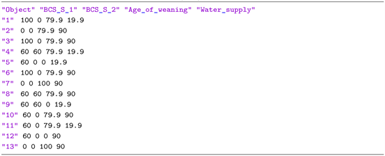
For the latter, the user needed to prepare a file organized as follows. OoI denoted the rows and ’DA’ criteria denoted the colums. It was important, that the object and criteria names in the file match the names entered in “AniFair” by the user. For criteria with qualitative performance level, the fields of the table might exclusively hold performance level as defined by the user. For criteria with quantitative performance level, the fields of the table contained the originally collected data, which was internally compared with the defined quantitative performance level by “AniFair”. “AniFair” could manage, if the number or order of OoI, respectively, ’DA’ criteria differ between user entered information and file, and it deleted duplicates. For the ’Good feeding’ example the beginning of the corresponding file was depicted in Listing 1.

If still the upload was not successful, a window was opened that showed an example on how to prepare the file, and “AniFair” allowed the user to choose

Figure 5. Manual entering of scores for OoI. A notebook with one tab per OoI was opened. On each tab the ’DA’ criteria were listed with drop down menus holding all performance level. In this example the OoI ’7’ was scored with performance level ’8.7 - 18.6’, ’0’, ’28 - 24.5’, and “0” for ’BCS_S_1’, ’BCS_S_2’, ’Age_of_weaning’, and ’Water_supply’, respectively.

another file or to switch to manual entering of object scores. For the manual entering of scores a notebook object with one tab per OoI was opened. On every tab the ’DA’ criteria were listed with drop down menus holding the performance level (Figure 5), so that the user could put together the collection of performance level associated with the respective OoI.

As the performance level of the criteria corresponded to scores on the final criteria scales $S_1^{\text{final}}\mathrm{,}\cdots \mathrm{,}{S}_n^{\text{final}}$, the collections of performance level associated with the OoI were transformed into vectors of scale entries between 0 and 100 within “AniFair”. These vectors formed the rows of an $m\times n$ matrix $\text{Scores}\left(\text{OoI}\right)$ with one row per OoI and one column per criterion.

2.5.3. Choquet Integral Aggregation

There were several mathematical approaches to identify a k-additive capacity (Section 2.4, Definition 6) reflecting specific user given information. An overview on the methods provided by the R-package ’Kappalab’ [39] was given in Grabisch, Kojadinovic, and Meyer [40]. For the “AniFair” implementation the approach ’maximum split’ via the R-function lin.prog.capa.ident was chosen. With the ’maximum split’ the minimal difference between the overall utility of the OoI was maximized from a system of linear inequations (SLI). For this, the OoI needed to be ranked by a partial weak order, because lin.prog.capa.ident needed the differences in overall utility of the OoI as an input. As the final criteria scales were comparable and reflected user preferences, it was meaningful to calculate mean scores for the OoI and to sort the rows of the matrix $\text{Scores}\left(\text{OoI}\right)$ (Section 2.5.2, paragraph Scoring of objects of interest, Listing 7) according to these means. As the rows of $\text{Scores}\left(\text{OoI}\right)$ corresponded to the overall utility of the OoI, one inequation was derived from two successive rows, comparing one OoI with the next best preferred OoI (Listing 2). Additionally, a preference threshold ${\delta }_C$ was set.

The R-function lin.prog.capa.ident was based on linear programming and used the R-package ’lpSolve’. Given the input Acp created in Listing 2, an object of class Mobius.capacity was created which held the capacity $\mu$ as list of coefficients. $\mu$ could afterwards be used to calculate the corresponding Choquet integral (Definition 4) using the function Choquet.integral (Listing 3).

Visualization of the Choquet results of pre-aggregation steps. In case of dependent subcriteria, “AniFair” opened a notebook with one tab for each criterion that had dependent subcriteria (Figure 6(a)). In each tab a table was presented. Let n_dep be the number of dependent subcriteria for the respective criterion, then the table had n_dep + 2 or n_dep + 3 columns. In the first column, the objects were listed. The following n_dep columns held the scores of the objects for the dependent subcriteria, i.e. the respective columns of the matrix Scores (OoI) (Section 2.5.2, paragraph Scoring of objects of interest). These were followed by a column for the mean scores and one column for the Choquet integral values if existent. The displayed results equaled the solution as provided by lin.prog.capa.ident without additional constraints on the Shapley value or the interaction (Listing 3). In order not to complicate the workflow the definition of constraints (compare paragraph Application of constraints and re-calculation) and the calculation of a weighted mean were not supported for pre-aggregation steps. The main aggregation step needed to be initiated by the user by clicking ’OK’.

Visualization of the Choquet results of the main aggregation and adding of constraints. For the main aggregation step, the results of Choquet integral calculation, the Shapley value, and the matrix of interaction indices were visualized in a window comprising three separated tables. If no dependent subcriteria

Figure 6. (a) Results of the pre-aggregation step of the dependent subcriteria ’BCS_S_1’ and ’BCS_S_2’ within the criterion ’BCS_S’. The table lists the OoI (first column) according to the averaged criteria scores (second last column). Scores for the aggregated subcriteria are given in columns two and three. The last column holds the values for the Choquet integral. (b) “AniFair” window presenting the results of the main aggregation step. The ’DA’ criteria ’Age_of_weaning’ and ’Water_supply’ as well as the pre-aggregated scores for the criterion ’BCS_S’ were averaged (second last column) and Choquet integral values were calculated. Underneath, the Shapley value is presented. At the bottom the interactions between the criteria are displayed.

were present, the matrix Scores (OoI) was included in the table at the top as the columns holding the scores for the OoI. In case of dependent subcriteria, the columns for these subcriteria were replaced by one column containing the pre-aggregated results for the respective first level criterion (Figure 6(b)). Again, the solution as provided by lin.prog.capa.ident without additional constraints on the Shapley value or the interaction was displayed. However, at the bottom of the results window the ’Add constraints on Shapley value and interaction’ button could be found.

No Choquet integral solution: Weighted mean as alternative. In the case no solution existed for the capacity, no Choquet integral values could be calculated. In the main aggregation, “AniFair” then proposed the calculation of a weighted mean as an alternative and provided the opportunity for the user to define or alter weights for the criteria. The results were presented in a table with a column for the weighted mean instead of the Choquet integral values (supplementary material, FigureS.7).

Application of constraints and re-calculation. The ’Add constraints on Shapley value and interaction’ button opened a notebook with four tabs, as two types of constraints could be defined for both Shapley value and interaction between criteria. On the one hand, for the Shapley and interaction indices interval boundaries between 0 and 1, respectively, −1 and 1 could be set. On the other hand, pre-orders could be defined, whereby the corresponding notebook tabs presented interactive matrices. In case of the Shapley indices, the criteria were displayed along the rows and the columns (Figure7). Right mouse click opened a drop down menu holding the choices ’=’, ’<’, and ’>’ associated with the constraint that the Shapley index of the criterion naming the row should be equal, lower or greater than the Shapley index of the criterion naming the column. In case of the interaction indices all pairs of criteria (i.e. ’BCS_S’-’Age_of_weaning’, ’BCS_S’-’Water_supply’, ’Age_of_weaning’-’Water_supply’) were displayed along the rows and colums (supplementary material, FigureS.5(c)). Again, the relation between the interaction indices of the criteria pairs could be evaluated as ’=’, ’<’, and ’>’ in drop down menus. Preference thresholds δ_S, δ_I were defined, and matrices Asp/Asi (for Shapley value), and Aip/Aii (for interaction) were generated for the formalization of the constraints. For every constraint that defined an interval one line consisting of the index (or indices in case of the interaction between two criteria) and the interval boundaries was added to Asi, respectively, Aii (Listing 4).

For every constraint defining the pre-order of Shapley or interaction indices two lines (equality of indices) or one line were added to Asp or Aip according to Listing 5.

Figure 7. Adding of constraints for the capacity calculation. A notebook with four tabs was opened. The tabs contain possibilities to define constraints on the Shapley value and the interaction between criteria. The constraints for both concepts can be entered by defining a pre-order or by specifying intervals in which the respective Shapley or interaction index should range. The above example displays the definition of a pre-order on the Shapley indices.

The pre-order of the OoI given to lin.prog.capa.ident via the argument Acp (Listing 2) was based on the assumption that all criteria were equally important to the decision problem. In re-calculation the pre-order needed to be reconsidered, when constraints on the Shapley value were defined that suggested otherwise. The generation of a weight vector representing the defined Shapley value constraints was implemented using the function lp from the R-package ’lpSolve’. A weighted version of the matrix Scores (OoI) of scores for the OoI was calculated while the weight vector was element wisely multiplied to the rows. From this weighted version of Scores(OoI) a weighted version of Acp was created according to Listing 2 and passed to lin.prog.capa.ident for the re-calculation (Listing 6) together with the constraints defining matrices Asp, Asi, Aip, and Aii.

As far as a solution existed that satisfied the given constraints, the results were displayed in a two-sided window (supplementary material, FigureS.6). On the left the solution from the preceding calculation was presented, and on the right the re-calculated solution could be seen. If no solution existed, the user was asked to define less strict constraints.

Figure 8. (a) The instances for ’Good feeding’, ’Good housing’, ’Good health’, and ’Appropriate behaviour’ are presented as tabs. In addition, here one tab is a remainder of a ’Deleted instance’. The ’AGGREGATION’ button started a Choquet integral aggregation of all instances that have not been deleted. (b) For all instances, a drop down menue held the available results (Choquet integral values or (weighted) mean). The user needed to choose which type of result should be used in the aggregation of instances. (c) For an easier representation the topics were automatically abbreviated to ’Good0’, ’Good1’, ’Good2’, ’Appro’ and the results of the aggregation of instances were displayed as table with one column for the scores of each instance, the mean scores and Choquet integral solutions or weighted mean.

Export of results. The windows displaying the results of aggregations were equipped with an ’Export’ button, in order to export the results to txt files (supplementary material, Listing Exported.3, Exported.5) and csv files (supplementary material, Listing Exported.4, Exported.6).

2.5.4. Aggregation of Instances

In the ’Multiple instances’—version of ’AniFair’ the instances appeared as tabs in the main window (Figure 8(a)). Every instance was handled as described in Sections 2.5.1, 2.5.2, and 2.5.3. As soon as results for the OoI existed for all instances, a Choquet integral aggregation of the instances could be initiated by clicking the ’AGGREGATION’ button. As could be seen in Figure 8(b), the user was presented with the type of results available for each instance: Choquet integral values or (weighted) mean. The results of the aggregation of instances were displayed in the same manner as the results for aggregation within instances (Figure 8(c)). Also, constraints on Shapley value and interaction indices could be defined, if a Choquet integral solution existed, and a weighted mean could be calculated, if no solution for the Choquet integral was given.

2.5.5. Application of ’AniFair’ to ’Good Feeding’ in ’Sows and Piglets’

Creation of criteria tree. In the “AniFair” instance in the first tab (Figure2) the topic ’Good feeding’ was entered as root for the criteria tree. Furthermore, the thirteen farms were entered as objects ’1’, ..., ’13’ as well as the first level criteria ’BCS_S’ (body condition score of sows), ’Age_of_weaning’, and ’Water_supply’. ’BCS_S’ was split up in second level criteria ’BCS_S_1’ and ’BCS_S_2’. As ’DA’ criteria the second level criteria ’BCS_S_1’ and ’BCS_S_2’ and the first level criteria ’Age_of_weaning’ and ’Water_supply’ were marked. As BCS was scored on a three-point scale and ’BCS_S_0/1/2’ were measured in percentages of affected animals, all information concerning ’BCS_S_0’ was given with the information on ’BCS_S_1’ and ’BCS_S_2’. A visualization of the complete criteria tree can be found in supplementary material (FigureS.1). The second level criteria ’BCS_S_1’, and ’BCS_S_2’ were marked dependent after “Proceed calculation” was hit (supplementary material, FigureS.2, Listing Exported.1).

Making criteria comparable. The definition of performance level, the filling of the matrices of judgment, and the adaption of the scales were carried out by the same person, who collected the data. The proper scientific background in the topic of animal welfare was guaranteed in the decision process. The bases of comparison were set to ’Quantitative performance level’ for the ’DA’ criteria ’BCS_S_1’, ’BCS_S_2’, and ’Age_of_weaning’. Being measured as percentages of sows and numbers of days, these criteria were scored on numerical scales (section 2.2). Performance level were inserted in order of decreasing attractiveness. The BCS value ’1’ was given to sows that failed the healthy state, therefore, it was desirable to have low percentages of sows with BCS ’1’. The three performance level ’<8.7’, ’8.7-18.6’, and ’>18.6’ were defined. ’2’ was the least desirable BCS value, as it described malnourished sows. The performance level defined here were ’0’, ’0-0.3’, and ’>0.3’. For ’Age_of_weaning’ averaged number of days from birth to weaning were grouped into the three performance level ’>28’, ’28-24.5’, and ’<24.5’. As ’Water_supply’ was measured qualitatively by judging the cleanliness and functionality of the drinkers, ’Qualitative performance level’ was set. The descriptions ’0: adequate’ and ’2: cleanliness and/or functionality not adequate’ were entered with the abbreviations ’0’ and ’2’. Pictures of the inserted performance level and the graphical visualizations of the adapted scales could be found in the supplementary material (Figures S.3, respectively, S.4). All user defined information was exported to txt file and could as well be found in the supplementary material (Listings Exported.1 and Exported.2). The OoI were afterwards scored by uploading the information from the file depicted in Listing 1 and the following 13 × 4 matrix $\text{Scores}\left(\text{OoI}\right)$ was build (Listing 7).

Choquet integral aggregation. Figure6 shows the results for the Choquet integral calculation. Additional constraints were defined afterwards. The criterion ’BCS_S’ was a so called animal-based measure [28]. WQAP recommended that in the evaluation of animal welfare a strong focus should lie on animal-based more than resource-based or management-based measures. Therefore, the user decided to define the following constraints regarding the Shapley value: Shapley index of ’BCS_S’ should be greater than the Shapley index of both ’Age_of_weaning’ and ’Water_supply’. A tolerance ${\delta }_S=0.01$ was given in the software. The user additionally defined constraints concerning the interaction among criteria. All criteria were considered complementary and the interaction among ’BCS_S’ and ’Age_of_weaning’, respectively, ’Water_supply’ should coincide. All constraints were presented in further detail in the supplementary material (FigureS.5). The constraints were applied, capacity and Choquet integral values were re-calculated and then exported to txt file (supplementary material, Listing Exported.3) and csv file (supplementary material, Listing Exported.4).

Aggregation of instances. As can be seen in Figure 8(c), ’AniFair’ instances for the animal welfare principles ’Good feeding’, ’Good housing’, ’Good health’, and ’Appropriate behaviour’ (automated abbreviations ’Good0’, ’Good1’, ’Good2’, ’Appro’) have been run, and an aggregation of the four principles was performed leading to a ranking of the thirteen farms according to an overall welfare score. As for ’Good health’ no Choquet integral values existed, for the sake of homogeneity the unweighted mean was chosen for all welfare principles in this example. The following constraints were defined, additionally: All interaction indices were limited between 0 and 1 to enforce independence or complementary interaction between the welfare principles. Via the pre-order of the Shapley indices equality of all Shapley indices was determined. The results as well as the associated Shapley value and interaction indices were exported to txt file (supplementary material, Listing Exported.5) and csv file (supplementary material, Listing Exported.6). Table 2 shows the results of the final Choquet integral calculations.

3. Results

According to user information, the following final scales were received for the “DA” criteria (supplementary material Listing Exported.2):

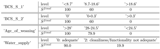
The scores of the 13 farms under analysis with respect to these scales can be found in Table 1. The Choquet integral values ranged from 9.33 to 72.78 with the proposed ’maximum split’ solution (Figure 6(b)). The Shapley value was $v=\left(\mathrm{0.3,0.36,0.34}\right)$ and interaction indices ranged from 0.11 and 0.28. Differences in Choquet integral values between consecutive farms averaged to 5.29 (±2.76). The final solution of the application of “AniFair” to ’Good feeding’ was associated with the Shapley value $v=\left(\mathrm{0.67,0.18,0.14}\right)$ and the interaction indices for all pairs of criteria equal 0.11. Table 1 shows the results of the final Choquet integral calculations. Choquet integral values ranged from 17.27 to 64.55, and the differences in Choquet integral values between consecutive farms averaged to 4.11 (±4.86). The farms could be separated into five groups with comparable overall ’Good feeding’ performance: farm ’8’; farms ’4’, ’3’, ’6’; farms ’1’, ’10’, ’9’; farm ’11’; farms ’12’, ’7’, ’13’, ’2’, ’5’.

Apart from the results delivered by “AniFair”, the part of the Choquet integral values which can be attributed to criteria interaction calculated according to Formula 7 (Section 2.4) can be found in the last column of Table 1. The proportion of the interaction ranged from approximately 5% of the Choquet integral value (farm ’8’) to approximately 55% (farms ’7’ and ’13’).

The final solution with regard to the aggregation of instances was associated with the Shapley value $v=\left(\mathrm{0.25,0.25,0.25,0.25}\right)$ and for all pairs of welfare principles the interaction indices equaled zero as set by the user. Choquet integral values ranged from 39.02 to 72.63 and coincided with the mean of the

Table 1. Results of the final Choquet integral calculations. The thirteen farms are listed in column 2 with respect to the ranking by the Choquet integral values (column 7). The scores of the farms regarding the final criteria scales are presented in columns 3 to 5. Additionally, the part of the Choquet integral values which can be attributed to criteria interaction can be found in the last column.

Table 2. Results of the aggregation of the welfare principles ’Good feeding’, ’Good housing’, ’Good health’, and Appropriate behaviour. The thirteen farms are listed in column 2 with respect to the ranking by the Choquet integral values (column 8). The scores of the farms regarding the principles are presented in columns 3 to 6.

scores due to vanishing interaction indices (Table 2). An image of the full screen visualizing the solution proposed by “AniFair” and the recalculation could be seen in supplementary material (FigureS.8).

4. Discussion

In the present article, the software tool “AniFair” for Multi-criteria decision analysis was introduced and presented via an example of assessing animal welfare with regard to the principles and criteria from the Welfare Quality® Assessment protocol for pigs. In contrast to ’Growing and finishing pigs’, no proposal for an aggregation system regarding ’Sows and piglets’ has been released yet [28]. The welfare principal ’Good feeding’ in ’Sows and piglets’ was chosen as the main example to present the functionality of “AniFair”, because it was less likely that a direct comparison with a currently used aggregation system could cloud the judgment of the possibilities offered by “AniFair”. As interims result, the thirteen farms that participated in data collection were associated with a ’Good feeding’ score (Table 1). Additional “AniFair” instances were applied to the principles ’Good housing’, ’Good health’, and ’Appropriate behaviour’ to illustrate the ’Multiple instances’—versions of “AniFair” and to aggregate the principle scores to overall welfare assessments for the farms.

To establish a ranking of the farms considering all criteria associated with ’Good feeding’ was a difficult task. The decision maker was forced to compare and weight multilayered information, as both quantitative criteria (’BCS_S_1’, ’BCS_S_2’, ’Age_of_weaning’); however on incomparable scales, and the qualitative criterion ’Water_supply’ needed to be taken into account. The MACBETH approach [10] was utilized to generate comparable scales from 0 to 100 based on user preferences in form of qualitative evaluations concerning differences of attractiveness. Instead of having to give quantitative information regarding his or her preferences, the user was confronted to qualitatively judge the differences between only two performance levels of a criterion at a time. The functionality described up to here was similarly implemented within the M-MACBETH software [11].

Looking at other methods in multi-criteria decision, the UTA (UTilités Additives) method proposed by Jacquet-Lagreze and Siskos [23] enables the estimation of a nonlinear additive function from the decision makers global preferences [41]. “AniFair” was implemented as part of a research project related to animal welfare. The meaningful addressing of animal welfare is currently an actively studied field; thus, global a priori preferences for a reference set would lack objectivity and compromise the transferability of the measurement principle. In UTA, during the assessment of a utility function, the interval between the extreme values of each criterion is partitioned into equally long subintervals [23]. This can only be done with quantitatively measured criteria, but in “AniFair” it was necessary to consider also qualitatively measured criteria. Furthermore, as the modeling of criteria interaction was desired, the Choqet integral was set as aggregation function in “AniFair”, whilst aggregation was integrated within the utility function regarding the UTA method. In comparison between the MACBETH approach and the AHP (Analytical Hierarchy Process) method [42], both provide means to structure the decision problem via a criteria tree, and both use a questioning-answering-protocol to help the user specify his or her preferences [43]. Although it would have been possible to combine the generation of criteria scales from AHP with the Choquet integral the same way the MACBETH approach and the Choquet integral were combined in “AniFair”, MACBETH was chosen over AHP. Reasons for this were the usage of the 9-point numerical scale in AHP compared to the semantic scale from MACBETH, and the differences in dealing with inconsistencies in the user judgment. Due to the 9-point numerical scale used in the AHP method, the decision maker has to quantify the differences of importance between pairs of options. Especially in cases of qualitative criteria, these differences might not be addressed properly by the given numerical options. In the MACBETH approach, the qualitative attributes are represented by six variables in the SLI [38], i.e. their quantity is based on how they were used by the decision maker. With the AHP method Eigenvalue methods on the matrix of user judgments were applied to calculate i.a. a consistency index which is thresholded at 0.1 to rate the user judgment as consistent, whilst in the MACBETH approach inconsistency is given when the SLI has no solution. As the comparability between criteria was one of the main tasks in the addressing of animal welfare, the authors figured it important to base the scales on consistent judgment without tolerances. Overall, the MACBETH approach seemed to be the most suitable method to achieve comparability.

However, in the M-MACBETH software, a questioning-answering-protocol was analogously used to determine criteria weights for the additive aggregation function. “AniFair” used the MACBETH approach solely to generate scales on which the criteria can be addressed comparably, but not for the weighting of criteria. As another difference, on every aggregation level within “AniFair” the Choquet integral [13] [40] was used as aggregation function replacing an additive aggregation, i.e. weighted mean. However, the weighted mean was presented as alternative, in case no solution for the Choquet integral existed. Furthermore, “AniFair” was built for applications where data for the OoI has been gathered in advance for all criteria considered in decision making (“DA” criteria). For the calculation of a capacity, a direct ranking of the OoI by the user was avoided in favor of a ranking strictly by the collected data to maintain objectivity (Section 2.5.2, Scoring of objects of interest). In applications with the necessity to prevent subjective influence in the ranking of objects, such as animal welfare, the approach proposed in “AniFair” might be more adequate than methods dealing with a user given pre-order e.g. additive or non-additive robust ordinal regression [44] [45]. In Clivillé, Berrah, and Mauris [22] the Shapley value and the interaction indices were determined from additional user preferences prior to capacity calculation. In contrast, as with the method proposed in Angilella, Greco, and Matarazzo [45] the “AniFair” approach worked with partial information, i.e. the user was not forced to specify his or her preferences concerning the importance of criteria or interaction between criteria to achieve a solution.

For the capacity calculation, the ’maximum split’ method was chosen that led to dispersed utilities and reached the maximal split that a Choquet integral solution can take for the given pre-order of objects [40]. This was considered the most suitable solution for users unfamiliar with capacity calculation or the theory behind multi-criteria decision making. Nevertheless, the user was afterwards invited to refine the proposed solution based on his or her knowledge about the relative importance of the criteria (i.e. Shapley value) and on how interaction between the criteria contributed to the decision problem. The Choquet integral was based on a capacity on the set of all criteria (Definition 3; Grabisch [14]). Thus, in assigning the relevance of a single criterion CRIT not only the value of the capacity of the one element set {CRIT} but the capacity values of all subsets containing CRIT needed to be considered (Section 2.4.1). The user had to be aware that all criteria combinations that included CRIT were weighted by setting constraints on the Shapley index of CRIT. In the ’Good feeding’ example, the Shapley value (Figure 7) was set according to the user preference that the criteria linked to animal-based measures should have a higher relative importance [28]. As a result, the Shapley index of ’BCS_S’ was ≈4.2 times higher than the Shapley indices of ’Age_of_weaning’ and ’Water_supply’ in the re-calculated solution (Section 2.5.5, Choquet integral aggregation). This changed the ranking of farms. Farm ’4’ was scored differently in the criteria compared to farms ’3’ and ’6’, but was also positioned second in the ranking due to the high relative importance of ’BCS_S’. For the same reason farms ’1’ and ’9’ improved in ranking whilst farm ’13’ dropped down five places. Although ’BCS_S’ was weighted highest by the user, the largest differences (between farms ’8’ and ’4’ as well as farms ’6’ and ’1’) were associated with changes in the score for ’Water_supply’. This was due to the fact, that ’Water_supply’ only had two performance level that were scored very differently (90.0 and 19.9), and gave rise to the question if this criterion might be resolved finely enough for the assessment of animal welfare. This illustrated the vulnerability of aggregation results towards relative importance of criteria. Scientific work [46] [47] proved that not only personal knowledge and topicality but various other factors influenced how the user evaluated the relevance of criteria.

Since independence of criteria usually was not given with real live decision problems [48], and since criteria interaction might be experienced differently among users [49], the possibility to model interaction between criteria was an important feature of “AniFair”. An example on how the aggregation of interacting criteria could not be modeled by a weighted mean could be found in Čaklović [50]. Only the interaction between pairs of criteria—associated with 2-additive capacities—was implemented in “AniFair” due to simplicity and the more likely existence of the mathematical solution. Additionally, the 2-additive case was the most interesting for practical applications [48]. Furthermore, it was less complicated to evaluate for the decision maker than interactions of higher order. As the welfare of pigs with regard to ’Good feeding’ was sensitive towards prolonged hunger as well as prolonged thirst (Section 2.1), the importance of the union of criteria was considered larger than the importance of single criteria, and thus, all criteria interacted positively (complementary criteria). Beneath others, in Table 1 the parts of the Choquet integral values that were associated to interaction were given. Farm ’8’ was ranked highest and showed high scores for all criteria. As a consequence only 5% of the overall ’Good feeding’ performance resulted from the interaction. On the contrary, for farms ’7’ and ’13’ the interaction represented approximately 55% of the farms performance, due to the large differences in criteria scores. It has to be noted, that without considering interaction these farms would have scored 30.93 and would, thus, have been ranked higher than farm ’12’ (29.93 without considering interaction). In addition to the successful combination between MACBETH and the Choquet integral (“AniFair”; Martín, Traulsen, Buxadé, and Krieter [30]; Clivillé, Berrah, and Mauris [22]), the importance of the modeling of interaction was undermined by Gomes, Machado, Costa, and Rangel [51], as they presented significant advances that arose from extending the TODIM (an acronym in Portuguese of Interactive and Multicriteria Decision Making [52]) method by using the Choquet integral as an aggregation function.

A further consequence of the recalculation, concerns the distribution of Choquet integral values. The ’maximum split’ solution was associated with fairly balanced weighting between the criteria. After recalculation, the range of Choquet integral values was narrower, the mean difference between consecutive farms was smaller, and the differences showed stronger variation. Instead of nearly equidistantly ranked farms with the ’maximum split’ solution, after the recalculation the distribution showed a majority of negligible differences. In this way, the more specific adaption of the model to user preferences in terms of constraints, led to a clear separation into groups of farms with comparable overall ’Good feeding’ scores, while the first farm in ranking farm ’8’ was clearly superior to the following farms. Thus, a more pronounced statement towards the animal welfare status was made.

Similar to the aforementioned AHP method, with ’AniFair’ at least two aggregation level were possible. With this the natural human tendency was supported to break down selection processes and to split up decision making in several stages, when the number of objects increased [53]. In the ’Good feeding’ example, a pre-aggregation from the second level criteria “BCS_S_1” and ’BCS_S_2’ to the first level criterion ’BCS_S’ had to take place, because ’BCS_S_1’ and ’BCS_S_2’ were considered dependent (Section 2.5.1, Independent and dependent subcriteria.). ’AniFair’ automatically initiated this pre-aggregation step and provided the aggregated ’BCS_S’ scores for the main aggregation. “AniFair” could in this regard be seen as a hybrid between AHP and MACBETH, as subcriteria can be aggregated to first level criteria like in AHP, but can also serve on equal terms to the first level criteria. In the latter case, the first level criteria play the role of ’Non-criteria nodes’ as in the M-MACBETH software and contribute only to the structuring of the decision problem but not to the decision process. Using the ’Multiple instances’—version of “AniFair”, the user was given an additional aggregation level by running multiple “AniFair” instances and applying the aggregation of instances.

All information were entered in “AniFair” via Graphical User Interfaces. The user was guided through the decision process, and his or her content-related expertise was specifically queried when needed for the next step in decision making. Behind the red ’?’ buttons that were placed in all windows where user interaction was needed (Figure 2, Figure 3, Figure 6, supplementary material Figures S.1-S.4) explanations on the necessary next steps could be found. For good usability the possibility to save and restore “AniFair” statuses as well as to upload data concerning the OoI from file was implemented (2.5.2, Saving and reloading “AniFair” status, Scoring of objects of interest). The txt files holding user entered information or results served to follow the choices made and constraints set by the user during the application of “AniFair” and to discuss his or her decision making among experts in the respective field. As the results were, additionally, exported as table to csv file (supplementary material Listings Exported.4 and Exported.6) and could easily be imported into statistical software, further analyses could be conducted. In contrast, the M-MACBETH software exports mcb files. The mcb file type is an uncommon data type and primarily associated with Glib Ravekit File2. As suitable software to open or convert mcb files programs as Glib Ravekit File, NEPLAN3 Project File or universal data viewer as FileMagic⁴ are needed.

Regarding animal welfare, the main concern is its measurability, as a clear definition as well as how to address animal welfare with overall scores are heavily discussed topics and subjects to current scientific research [26] [28] [30]. Animal welfare is on the one hand bound to moral questions and prone to emotional discussion but on the other hand connected to economical questions as well as social and political aspects. Compared to decision problems concerning personal life or structural decisions and improvement in companies, subjectivity needs to be applied with all care. As a matter of fact, the impact of considering multiple decision criteria in assessing animal welfare was once more underlined by the fact that the ranking of farms had changed comparing the ’Good feeding’ scores with the overall welfare scores including all four principles. A special example was farm ’13’, that was ranked highest in the overall welfare score but was found only on the eleventh rank when the analysis was reduced to ’Good feeding’. On the contrary, farm ’4’ was ranked second with regard to “Good feeding” and took position eleven in the ranking due to the results of the aggregation over all welfare principles. Exemplarily, farms ’9’, ’10’, ’11’ hold ranks six to eight in both aggregations (Table 1, Table 2). As a consequence, for an overall welfare score all four principles should be evaluated to come to a holistic welfare assessment. The origination of the overall scores was transparent, as “AniFair” provided Shapley value, interaction indices and all interims results such as pre-aggregation results and information on how the individual farms scored in the criteria. With this, farmers could be shown their current animal welfare status compared to other farms. As the criteria scales were made homogeneous and the relative importance of the criteria is known, “AniFair” results were a solid basis for aimed advice to the farms with low rankings, in which criterion it was most pressing to improve the welfare status. In a discourse between farmers, animal welfare scientists and politicians, the theoretical aspects of measuring animal welfare combined with the overall welfare scores with regard to real farms could attest or revise animal welfare assessment. A reliable overall welfare score could serve as a basis for the certification of animal welfare labels which allow consumers to choose their animal-related products with regard to good animal welfare.

Acknowledgements

Gratitude is expressed to the farmers that participated in the data collection.

Formatting of Funding Sources

This work was supported by the Federal Ministry of Food and Agriculture (funding code 2817200913).

Supplementary Material

On the Chosen Example

Animal welfare has gotten in the public eye and has become an important issue for consumers. Politics has come up with various legal requirements for the farmers to look after and maintain the welfare status of their animals. To avoid emotionality in the discussion about this topic, it became essential to clearly define the terminology and to provide a conceptually sound assessment of animal welfare. For this reason scientific work has been carried out inter alia by the Welfare Quality® project. The latter identified twelve welfare criteria that were partitioned in the four welfare principles ’Good feeding’, ’Good housing’, ’Good health’, and ’Appropriate behaviour’. The assessment of animal welfare according to Welfare Quality® was based on multiple indicators which—in the form they are gathered—were not necessarily comparable, but measured as binary decisions, on three-point scales or on cardinal scales. Comparability of the collected information was achieved by decision trees, index calculation, and I-spline functions, before the scores were stepwisely aggregated to an overall evaluation of the welfare standards of farms (Welfare Quality® 2009a; Welfare Quality® 2009b; Welfare Quality® 2009c).

When it came to the welfare of pigs, Welfare Quality® proposed aggregation systems for ’Growing and finishing pigs’ based on the above mentioned methods which were implemented in an online calculator^S1 to achieve overall welfare scores. For ’Sows and piglets’ no proposal for an aggregation system has been released yet. The authors chose ’Sows and piglets’ in terms of the welfare principal ’Good feeding’ as the main example to present the functionality of “AniFair”, because it was less likely that a direct comparison with a currently used aggregation system could cloud the judgment of the possibilities offered by “AniFair”. Furthermore, “AniFair” provided the choice between a ’Single instance’—and a ’Multiple instances’—version. The remaining three welfare principles were used to present the ’Multiple instances’—version and the possibility to aggregate over multiple instances, but those were neither discussed nor illustrated in detail.

^S1http://www1.clermont.inra.fr/wq/index.php?id=simul&new=1.

An expert in animal welfare collected the data and made all decisions regarding criteria performance level, the differences of attractiveness between them, the modification of precardinal scales and the definition of constraints. However, it was not the intent of the main article to discuss the meaning of the user entered information or the resulting ranking of farms as final truth concerning the assessment of pig welfare. Rather should “AniFair” be introduced as a tool to address the assessment of e.g. animal welfare in a transparent way.

As not all user entered information or results could have been displayed in the main article, missing visualization for the ’Good feeding’ example as well as graphical illustrations concerning the aggregation over all four instances ’Good feeding’, ’Good housing’, ’Good health’, and ’Appropriate behaviour’ was placed in this Supplementary material.

“AniFair” Application to ’Good Feeding’ in ’Sows and Piglets’

Creation of criteria tree. Assessed were the welfare criteria ’Absence of prolonged hunger’ and ’Absence of prolonged thirst’ (main article Section 2.2.1) via the measures body condition score of sows (’BCS_S’), age of weaning (’Age_of_weaning’), and water supply (’Water_supply’). ’BCS_S’ was divided into the second level criteria (subcriteria) ’BCS_S_1’, ’BCS_S_2’. At data collection the percentages of sows scored ’1’, and ’2’ were calculated for every farm. The criterion ’Age_of_weaning’ was assessed as the averaged number of days from birth to weaning as stated by the farmer. The criterion ’Water_supply’ was given by a binary decision, if the drinking places for sows and piglets were adequate regarding the cleanliness and functionality of all drinkers (score ’0’) or not (score ’2’). From these criteria a criteria tree was build in the “AniFair” main window which was fully displayed in FigureS.1. All criteria that were selected by the ’DA’ buttons were marked in bold and red font. Hitting the ’Proceed calculation’ button opened a GUI window where the User had to decide upon the in/dependence of subcriteria (main article Section 3.1, Independent and dependent subcriteria) and confirm the choices before further processing could be carried out (FigureS.2).

Making criteria comparable. In FigureS.3 the definitions of the performance level for the decision criteria were illustrated. As a next step, the matrices of judgment could be filled in (Appendix: Background of ’Making criteria comparable’). The evaluation of the differences of attractiveness could for all criteria be viewed in Listing Exported.1 together with the export of the criteria tree and the definition of performance level. All Listings were presented in the Appendix: Data exported from “AniFair” of this Supplementary material.

Based on these user preferences “AniFair” scales were calculated which were precardinal scales, i.e. the distances between the entries on the scale mirror the qualitative attributes with which the User evaluated the pairwise differences between performance level. However, the relative differences of attractiveness as experienced by the User might not be represented by distances between entries on the “AniFair” scales. That was why the User was asked to modify the scales after inspecting the graphical visualization. FigureS.4 illustrated the “AniFair” scales on the left and the final criteria scales after user modification on the right exemplary for ’Age_of_weaning’ and ’Water_supply’. As an example, the User experienced that the performance level ’28 - 24.5’ of criterion ’Age_of_weaning’ needed to be scored closer to the maximum score 100 associated with the performance level ’>28’ than “AniFair” had suggested. Thus, the User modified the scale for ’Age_of_weaning’ by raising the score for ’28 - 24.5’ via the spin buttons of the thermometer. “AniFair” internally calculated boundaries (Appendix: Background of ’Making criteria comparable’, Dependent intervals.) for the modification of the scale to prevent that the user preferences entered earlier were

Figure S.1. Fully filled in criteria tree. The thirteen farms have been entered as objects ’1’, ..., ’13’. As first level criteria ’BCS_S’, ’Age_of_weaning’ and ’Water_supply’ have been inserted. For ’BCS_S’ the second level criteria ’BCS_S_1’, ’BCS_S_2’ have been defined and marked as criteria for which data was available (’DA’ criteria). Additionally, ’Age_of_weaning’ and ’Water_supply’ have been specified as ’DA’ criteria.

Figure S.2. (a) For all criteria with second level criteria the User has to make the choice, if these subcriteria should be treated as dependent or independent. In case of independent subcriteria, the second level criteria (here: ’BCS_S_1’, ’BCS_S_2’) will be used in the main aggregation instead of ’BCS_S’ together with the first level criteria. Otherwise a pre-aggregation step for ’BCS_S_1’ and ’BCS_S_2’ within ’BCS_S’ takes place and the ’BCS_S’ results will be used in the main aggregation. (b) The User has to confirm the specification of criteria for which data was available (’DA’) and the choice regarding the (in) dependence of subcriteria.

violated (FigureS.4(a) & FigureS.4(b)). The “AniFair” scale for ’Water_supply’ consisted of a straight line from 100 to 0, because only two performance level were defined. One possible modification of this scale without violating the condition that the

Figure S.3. Readily defined bases of comparison and performance level. For all four ’DA’ criteria the basis of comparison has been set. ’Quantitative performance level’ has been chosen for ’BCS_S_1’ to ’Age_of_weaning’, respectively, ’Qualitative performance level’ for ’Water_supply’. Furthermore, performance level have been defined for all criteria.

User judged the difference of attractiveness between ’0’ and ’2’ as ’very strong’ would be to lower the score of ’0’ to 90.0 and raise the score of ’2’ to 19.9 as visualized in the example (FigureS.4(c) & FigureS.4(d)). For ’BCS_S_1’, ’BCS_S_2’, and ’BCS_S’ no user modifications were made. For the sake of reproducibility, all “AniFair” and final scales were exported to txt file and can be seen in Listing Exported.2 in the Appendix: Data exported from “AniFair”.

Choquet integral aggregation. For the calculation of the Choquet integral the User needed to provide “AniFair” with the information, how each of the thirteen farms performed with regard to the ’DA’ criteria. In this example this scoring of objects took place via upload from file (main article Section 3.2, Scoring of objects of interest).

The performance level assigned to the farms were transformed into scores on the final criteria scales and in a first run Choquet integral values were calculated without any additional constraints (main article Section 3.3, Visualization of the Choquet results of the main aggregation and adding of constraints.). In addition to the constraints with regard to the pre-order of the Shapley indices (main article Figure7, Section 3.3, Application of constraints and re-calculation.) the constraints displayed in FigureS.5 were defined. The User wanted the Shapley indices of ’BCS_S’ to be higher, because animal-based measures as ’Body condition score’ were considered more important in the assessment

Figure S.4. In the left column of (a) (b) and (c) (d) the scales are displayed in the graphic and the thermometer as calculated by “AniFair”. In the right column the scales have been modified by the User in a manner that his or her concept of relative attractiveness between criteria is fulfilled (Appendix: Background of ’Making criteria comparable’, Matrices of judgment and scale calculation, Dependent intervals). Boundaries within which the before made evaluation of differences of attractiveness stay fulfilled are internally calculated to make sure that the displayed scales are always consistent with the user defined preferences. (a) (b) For the criterion ’Age_of_weaning’ the score for the performance level ’24.5’ has been raised to the boundary, that is why the corresponding marker has changed appearance and color from circle to crossed square and from green to red. (c) (d) For ’Water_supply’ the score for ’0’ has exemplarily been lowered from 100.0 to 90.0 and the score for ’2’ has been raised from 0.0 to 19.9.

Figure S.5. User defined constraints for ’Good feeding’. Constraints concerning the pre-order of Shapley indices have already been presented in Figure 7 in the main article. (a) Interval boundaries for the Shapley indices have been entered. The indices with regard to ’Age_of_weaning’ and ’Water_supply’ have been limited by 0.3. (b) Intervall boundaries for the interaction indices have been entered. All pairs of criteria have been set to interact complementary as the interaction indices have been forced to be ≥ 0. (c) Conditions for a pre-order of interaction indices concerning pairs of criteria have been defined. All pairs have been set to interact equally.

of animal welfare (FigureS.5(a)). FigureS.5(b) showed, that all interaction indices had been set greater than zero. As the welfare of pigs was sensitive towards prolonged hunger as well as prolonged thirst, the importance of the union of criteria was considered larger than the importance of single criteria, and thus, all criteria interact positively (complementary criteria). Furthermore, the User considered it necessary, that the interaction indices for pairs of criteria coincided. These constraints were defined via the pre-order of interaction indices (FigureS.5(c)).

In FigureS.6 could be seen, that the ranking of farms with regard to the welfare principle ’Good feeding’ had changed for rank 2 and following. Furthermore, the Shapley value and the interaction indices had been adapted according to the defined constraints. The final results as well as the constraints were then exported to txt-file and csv-file (Listings Exported.3, Exported.4 in Appendix: Data exported from “AniFair”).

’Multiple instances’—version and aggregation of instances. ’Good feeding’ and the remaining welfare principles ’Good housing’, ’Good health’, and ’Appropriate behaviour’ were run out in the ’Multiple instances’—version of ’AniFair’ (main article Section 3.4). As with ’Good health’ no capacity solution existed and a weighted mean was calculated instead, these results were displayed in FigureS.7 as an example for the weighted mean alternative (main article Section 3.3, No Choquet integral solution: Weighted mean as alternative). However,

Figure S.6. Re-calculated solution for ’Good feeding’ after the application of constraints on Shapley value and interaction.

Figure S.7. (a) No capacity solution could be calculated for the welfare principle ’Good health’. The column for the Choquet integral values is missing. The place of the ’Add contraints on Shapley value and interaction’ button has been taken by the button ’Calculate weighted mean’. (b) After the User entered a weight vector the weighted mean has been represented instead of the Choquet integral values. Note that the order of the objects has changed during the calculation of the weighted mean.

Figure S.8. Re-calculated solution for the aggregation of instances after the application of constraints on Shapley value and interaction.

all other results and user entered information regarding the welfare principles ’Good housing’, ’Good health’, and ’Appropriate behaviour’ were not illustrated, as in this article no detailed discussion on the welfare of pigs but a presentation of the “AniFair” software tool was aspired.

For the aggregation of instances the User was presented with the type of results available for each instance (main article Section 3.4, Figure8(b)). As for ’Good health’ no Choquet integral values existed, for the sake of homogeneity the unweighted mean was chosen for all welfare principles in this example. The results of aggregation prior to the definition of constraints was displayed in Section 3.4, Figure8(c) in the main article. The following constraints had been defined, additionally: All interaction indices have been limited between 0 and 1 to enforce complementary interaction between the welfare criteria. Via the pre-order of the Shapley indices equality of all Shapley indices was determined. The results as well as the associated Shapley value and interaction indices were exported to txt file (Listing Exported.5 in Appendix: Data exported from “AniFair”) and could be viewed in FigureS.8.

As a result the thirteen farms were assigned overall scores for all individual welfare principals and an overall evaluation of the welfare standard. A ranking was formed that reflects the relative importance of the criteria, respectively, principles. As the scores were made comparable and displayed together with the final scores, aimed advice could be given to the farms with low rankings, in which criterion/principle it was most pressing to improve the welfare status of the animals. All decisions could be looked up in the exported files and served as basis for discussion for animal welfare experts.

Saving and reloading “AniFair” status. Up to three ’{SAVE}’ buttons could be found in “AniFair”. With these buttons the current “AniFair” status could be saved. This included OoI, criteria, subcriteria, information which criteria are ’DA’, information on the (in) dependence of subcriteria, bases of comparison, performance level, matrices of judgment, “AniFair” scales and dependent intervals. In contrast to the export of user entered information, scales or results to txt files, these “AniFair” status files were not designed for analysis or to be human readable, but to reload information into “AniFair”. Every “AniFair” instance was equipped with a ’LOAD’ button to restore all information in a respective “AniFair” status. Afterwards, criteria could be added without compromising any loaded information. However, the deletion of a criterion could compromise the mapping between the criteria and the information on performance level, matrices of judgment, scales and dependent intervals. “AniFair” might, thus, be obliged to ignore the information. Alteration of criteria also caused “AniFair” to neglect the information on the respective criteria.

Appendix 1

Appendix: Data exported from “AniFair”

Appendix 2: Background of ’Making Criteria Comparable’

Performance level. The term performance level referred to the different states that can occur regarding a criterion (Section 3.2 in the main article; Bana e Costa, Corte, and Vansnick (2003)). For qualitative criteria the performance level were characteristics like the colors of a car or existence versus non-existence of an illness. Quantitative criteria could be measured on a numerical scale like percentages of sick animals in a herd. With this, exemplary performance level could be ’0 - 10’, ’10 - 50’, ’>50’. After a list of ’DA’ criteria had been confirmed, “AniFair” opened a window with one framed box container for every criterion. Next to the criterion name a drop down menu was placed, in which the basis of comparison could be set either ’Quantitative performance level’ or ’Qualitative performance level’. In the quantitative case “AniFair” prepared two slots ’insert level 1’ and ’insert level 2’ (Figure 3(a) in the main article), because for each criterion at least two performance level should be defined. More slots could be produced by clicking ’Add...’. The ’insert level’ slots were editable so that numerical values (or intervals) can be entered as performance level. By removing the content, slots could be deleted. In the case of ’Qualitative performance level’ two columns of slots were prepared by “AniFair”. For the entering of performance level description there were slots ’insert description of level 1/2’, and in addition abbreviations for the level descriptions need to be entered in ’lev 1/2’.

Matrices of judgment and scale calculation. When performance level for a criterion CRIT were defined, the matrix of judgment needed to be filled in (Figure 4 in the main article). The User had to evaluate the DoA between pairs of performance level. These differences were assessed qualitatively with one of the six attributes ’extreme’, ’very strong’, ’strong’, ’moderate’, “weak’ and ’very weak’ BanaECostaVansnick99. Every pair of performance level was represented by a button showing ’?’. Right mouse click opened a drop down menu showing the above mentioned attributes. The additional option ’no’ corresponded to the case when the User evaluated the respective performance level as equally attractive. Given that $N_{CRIT}$ was the number of performance level defined for CRIT, the user judgments were transformed into a system of linear inequations (SLI) with $N_{CRIT}+6$ variables. The attributes ’very weak’, ..., ’extreme’ were represented by six additional variables ${\sigma }_1,\cdots ,{\sigma }_6$, respectively. By including the inequations $\mathrm{0\; <mo>\; <\; </mo>}{\sigma }_1$ and ${\sigma }_{l-1}\mathrm{<mo>\; <\; </mo>}{\sigma }_l$ for $l\in \left\{2,\cdots ,6\right\}$, it was made sure that the differences described by the attributes were increasing from ’no’ to ’extreme’. Exemplary, if for $i,j\le N_{CRIT}$ the judgment that the DoA between the $i^{th}$ and the $j^{th}$ performance level of CRIT was ’moderate’, the inequations ${\sigma }_3<x_i-x_j$ and $x_i-x_j<{\sigma }_4$ were included in SLI. If the User found the $i^{th}$ and the $j^{th}$ performance level equally attractive, the equation $x_i-x_j=0$ was included instead. A solution for SLI is calculated by the function lp from the R-package ’lpSolve’ lpSolve. The first $N_{CRIT}$ entries of the solution fulfilled Definition 2 in Section 2.3.1 of the main article and served as precardinal scale, i.e. the distances between the entries on the scale mirror the qualitative attributes with which the User evaluated the pairwise differences between performance level. A positive affine function was applied to set the maximal score on the scale to 100. This was associated to the most attractive performance level. The scales as calculated by “AniFair” for the n ’DA’ criteria were denoted $S_1^{\text{AniFair}},\cdots ,S_n^{\text{AniFair}}$.

Inconsistency. With every modification of the interactive fields in the matrix of judgment, the SLI changed and was checked regarding the existence of a solution. When the judgments appeared to be inconsistent with a precardinal scale, a modal dialog opened to help the User to solve the inconsistency. The dialog specified the judgment lastly made and showed a list of suggestions (Figure 4 in the main article). The words ’UP’ and ’DOWN’ were displayed in green and blue, if a DoA was suggested to be evaluated larger and smaller than the current judgment, respectively. This inconsistency warning disappeared as soon as the matrix of judgment was clicked again. It was possible that the inconsistency was not solved by changing one judgment or that a judgment had to be increased or decreased further than to the attribute describing the next greater or smaller DoA.

Dependent intervals. “AniFair” supported the refinement of the positions of scores on the precardinal “AniFair” scales in order to achieve cardinal scales (Section 2.3.1 in the main article). Repositioning could be carried out without violation of user preferences within the dependent interval of each score: We referred to the dependent interval associated to a score s on an “AniFair” scale $S_i^{\text{AniFair}}$, $i\le n$ as the interval between the minimal and maximal possible value for s such that $S_i^{\text{AniFair}}$ still reflected its underlying user preferences, given that all other scores on $S_i^{\text{AniFair}}$ were kept fixed. For the calculation of the dependent interval for s the conditions that all scores except s remain unchanged were included in the SLI described in paragraph Matrices of judgment and scale calculation. The function lp was then used twice to optimize the SLI with respect to minimal and maximal values of s. Dependent intervals were re-calculated with every user modification (paragraph Visualization and adaption of scales) of the “AniFair” scales.

Visualization and adaption of scales. A notebook opened with one tab per ’DA’ criterion to display the precardinal “AniFair” scales $S_1^{\text{AniFair}}\mathrm{,}\cdots \mathrm{,}{S}_n^{\text{AniFair}}$. On the left, the scale was shown as curve with the performance level labeling the horizontal axis. On the right, the scale was presented as thermometer, similar to the scale representation in the M-MACBETH software MMacBeth. The displayed scores in the thermometer were editable and could also be altered via spin buttons. Every altering of scores in the thermometer led directly to adaption of the graphic. In this way, the User could modify the “AniFair” scales within the dependent intervals (paragraph Dependent intervals). If the User for example evaluated all DoA between successive performance level equally, e.g by the attribute ’moderate’, the “AniFair” scale was presented by a straight line. However, all successive DoA could be ’moderate’ without the necessity of an equidistant scale, as ’moderate’ was a qualitative judgment and represented a range of DoA. The User could, thus, refine the relative DoA according to his or her experience. In this way final cardinal criteria scales $S_1^{\text{final}}\mathrm{,}\cdots \mathrm{,}{S}_n^{\text{final}}$ were obtained (Section 2.3.1 in the main article). While clicking the ’Ok’ button of the notebook, the User could export “AniFair” scales $S_1^{\text{AniFair}}\mathrm{,}\cdots \mathrm{,}{S}_n^{\text{AniFair}}$ as well as the final criteria scales $S_1^{\text{final}}\mathrm{,}\cdots \mathrm{,}{S}_n^{\text{final}}$ of all criteria to txt file and proceed to the scoring of objects. Figures of visualization and adaption as well as the exported txt file for the ’Good feeding’ example could be found in the Supplementary Material (FigureS.4, Listing Exported.2). The scales for criteria with dependent subcriteria were displayed the same way.

NOTES

¹Note that in general a particle could be present in more, not less, than n_directions subspaces. Is that the case, it is necessary because the discrete Planck’s constant applies to all types of particles to split n_particle in subsets of n_directions subspaces.

²https://filext.com/file-extension/MCB.

³https://www.neplan.ch.

⁴www.filemagic.com.

Conflicts of Interest

The authors declare no conflicts of interest regarding the publication of this paper.

References

[1]	Steuer, R.E. (1986) Multiple Criteria Optimization: Theory, Computation, and Application. Wiley Series in Probability and Mathematical Statistics. https://books.google.de/books?id=tSA%5C_PgAACAAJ https://doi.org/10.1002/oca.4660100109
[2]	Ho, W. (2008) Integrated Analytic Hierarchy Process and Its Applications—A Literature Review. European Journal of Operational Research, 186, 211-228. https://doi.org/10.1016/j.ejor.2007.01.004
[3]	Mardani, A., Zavadskas, E.K., Khalifah, Z., Jusoh, A. and Nor, K. (2015) Multiple Criteria Decision-Making Techniques in Transportation Systems—A Systematic Review of the State of the Art Literature. Transport, 31, 359-385. https://doi.org/10.3846/16484142.2015.1121517
[4]	De Castro, A.K.A., Pinheiro, P.R., Pinheiro, M.C.D. and Tamanini, I. (2011) Towards the Applied Hybrid Model in Decision Making: A Neuropsychological Diagnosis of Alzheimer’s Disease Study Case. International Journal of Computational Intelligence Systems, 4, 89-99. https://doi.org/10.1080/18756891.2011.9727766
[5]	Mardani, A., Zavadskas, E.K., Khalifah, Z., Zakuan, N., Jusoh, A., Nor, K. and Khoshnoudi, M. (2017) A Review of Multi-Criteria Decision-Making Applications to Solve Energy Management Problems: Two Decades from 1995 to 2015. Renewable and Sustainable Energy Reviews, 71, 216-256. https://doi.org/10.1016/j.rser.2016.12.053
[6]	Zavadskas, E. and Turskis, Z. (2011) Multiple Criteria Decision Making (MCDM) Methods in Economics: An Overview. Technological and Economic Development of Economy, 17, 397-427. https://doi.org/10.3846/20294913.2011.593291
[7]	Liou, J.J.H. and Tzeng, G.-H. (2012) Comments on Multiple Criteria Decision Making (MCDM) Methods in Economics: An Overview. Technological and Economic Development of Economy, 18, 672-695. https://doi.org/10.3846/20294913.2012.753489
[8]	Bana e Costa, C.A. and Vansnick, J.C. (1999) The MACBETH Approach: Basic Ideas, Software, and an Application. In: Meskens, N. and Roubens, M., Eds., Advances in Decision Analysis, Mathematical Modelling: Theory and Applications, Vol. 4, Springer, Dordrecht, 131-157. https://doi.org/10.1007/978-94-017-0647-6_9
[9]	Bana e Costa, C.A. (1992) Structuration, Construction et Exploitation d’un Modèle Multicritère d’Aide à la Décision. Lisbon.
[10]	Bana e Costa, C.A., de Corte, J.M. and Vansnick, J.C. (2003) MACBETH. Working Paper 03.56, London School of Economics, London. http://eprints.lse.ac.uk/22761/1/MACBETH_LSE_working_paper_0356_30set.pdf
[11]	Bana e Costa, C.A., de Corte, J.M. and Vansnick, J.C. (2017) M-MACBETH Version 2.5.0 User’s Guide. http://www.m-macbeth.com
[12]	Murofushi, T. and Sugeno, M. (1989) An Interpretation of Fuzzy Measure and the Choquet Integral as an Integral with Respect to a Fuzzy Measure. Fuzzy Sets and Systems, 29, 201-227. https://doi.org/10.1016/0165-0114(89)90194-2
[13]	Choquet, G. (1954) Theory of Capacities. Annales de l’Institute Fourier, 5, 131-295. https://doi.org/10.5802/aif.53
[14]	Grabisch, M. (1997) K-Order Additive Discrete Fuzzy Measures and Their Representation. Fuzzy Sets and Systems, 92, 167-189. https://doi.org/10.1016/S0165-0114(97)00168-1
[15]	Peters, J.F. and Ramanna, S. (1996) Application of the Choquet Integral in Software Cost Estimation. Proceedings of IEEE 5th International Fuzzy Systems, New Orleans, 8-11 September 1996, 862-866.
[16]	Ferreira, J.M., Jalali, M.S. and Ferreira, F.A.F. (2018) Enhancing the Decision-Making Virtuous Cycle of Ethical Banking Practices Using the Choquet Integral. Journal of Business Research, 88, 492-497. http://www.sciencedirect.com/science/article/pii/S014829631730526X https://doi.org/10.1016/j.jbusres.2017.12.031
[17]	Camargo, M., Fonteix, C. and Morel, L. (2006) Application of the Choquet Integral to a Chemical Manufacturing Process. IFAC Proceedings, 39, 282-286. http://www.sciencedirect.com/science/article/pii/S1474667015330640 https://doi.org/10.3182/20060522-3-FR-2904.00045
[18]	Shieh, J.I., Wu, H.H. and Liu, H.C. (2009) Applying a Complexity-Based Choquet Integral to Evaluate Students’ Performance. Expert Systems with Applications, 36, 5100-5106. https://doi.org/10.1016/j.eswa.2008.06.003 http://www.sciencedirect.com/science/article/pii/S0957417408003229
[19]	Liu, H., Wang, X. and Kadir, A. (2013) Color Image Encryption Using Choquet Fuzzy Integral and Hyper Chaotic System. Optik—International Journal for Light and Electron Optics, 124, 3527-3533. https://doi.org/10.1016/j.ijleo.2012.10.068 http://www.sciencedirect.com/science/article/pii/S0030402612008960
[20]	Mayag, B., Grabisch, M. and Labreuche, C. (2011) A Representation of Preferences by the Choquet Integral with Respect to a 2-Additive Capacity. Theory and Decision, 71, 297-324. https://doi.org/10.1007/s11238-010-9198-3
[21]	Berrah, L., Clivillé, V., Montmain, J. and Mauris, G. (2019) The Contribution Concept for the Control of a Manufacturing Multi-Criteria Performance Improvement. Journal of Intelligent Manufacturing, 30, 47-58. https://doi.org/10.1007/s10845-016-1227-9
[22]	Clivillé, V., Berrah, L. and Mauris, G. (2007) Quantitative Expression and Aggregation of Performance Measurements Based on the MACBETH Multi-Criteria Method. International Journal of Production Economics, 105, 171-189. http://www.sciencedirect.com/science/article/pii/S0925527306000739 https://doi.org/10.1016/j.ijpe.2006.03.002
[23]	Jacquet-Lagreze, E. and Siskos, J. (1982) Assessing a Set of Additive Utility Functions for Multicriteria Decision-Making, the UTA Method. European Journal of Operational Research, 10, 151-164. https://doi.org/10.1016/0377-2217(82)90155-2 http://www.sciencedirect.com/science/article/pii/0377221782901552
[24]	Grandin, T. (2013) Animals Are Not Things: A View on Animal Welfare Based on Neurological Complexity. Trans-Scripts 3: An Interdisciplinary Online Journal in Humanities and Social Sciences at UC Irvine. http://sites.uci.edu/transscripts/files/2014/10/2013_03_10.pdf
[25]	Gazzano, A., Giussani, S., Gutiérrez, J., Ogi, A. and Mariti, C. (2018) Attitude toward Nonhuman Animals and Their Welfare: Do Behaviorists Differ from Other Veterinarians? Journal of Veterinary Behavior, 24, 56-61. http://www.sciencedirect.com/science/article/pii/S1558787817302149 https://doi.org/10.1016/j.jveb.2018.01.006
[26]	Czycholl, I., Kniese, C., Büttner, K., Grosse Beilage, E., Schrader, L. and Krieter, J. (2016) Test-Retest Reliability of the Welfare Quality® Animal Welfare Assessment Protocol for Growing Pigs. Animal Welfare, 25, 447-459. http://www.ingentaconnect.com/content/ufaw/aw/2016/00000025/00000004/art00006 https://doi.org/10.7120/09627286.25.4.447
[27]	Welfare Quality® (2009) Welfare Quality® Assessment Protocol for Cattle. Welfare Quality® Consortium, Lelystad.
[28]	Welfare Quality® (2009) Welfare Quality® Assessment Protocol for Pigs (Sows and Piglets, Growing and Finishing Pigs). Welfare Quality® Consortium, Lelystad.
[29]	Welfare Quality® (2009) Welfare Quality® Assessment Protocol for Poultry (Broilers, Laying Hens). Welfare Quality® Consortium, Lelystad.
[30]	Martín, P., Traulsen, I., Buxadé, C. and Krieter, J. (2016) Development of a Multi-Criteria Evaluation System to Assess Growing Pig Welfare. Animal, 11, 466-477. https://doi.org/10.1017/S1751731116001464
[31]	Miele, M., Veissier, I., Evans, A. and Botreau, R. (2011) Animal Welfare: Establishing a Dialogue between Science and Society. Animal Welfare, 20, 103-117.
[32]	Evans, A.B. and Miele, M. (2012) Between Food and Flesh: How Animals Are Made to Matter (and Not Matter) within Food Consumption Practices. Environment and Planning D: Society and Space, 30, 298-314. https://doi.org/10.1068/d12810
[33]	Grabisch, M. and Roubens, M. (2000) Application of the Choquet Integral in Multicriteria Decision Making. In: Fuzzy Measures and Integrals, Physica Verlag, Berlin, 348-374.
[34]	Shapley, L.S. (1953) A Value for n-Person Games. In: Kuhn, H.W. and Tucker, A.W., Eds., Contribution to the Theory of Games, Vol. 2, Annals of Mathematics Studies 28, Princeton University Press, Princeton, 307-317. https://doi.org/10.1515/9781400881970-018
[35]	Murofushi, T. and Soneda, S. (1993) Techniques for Reading Fuzzy Measures (III): Interaction Index. Proceedings of the 9th Fuzzy Systems Symposium, Sapporo, 693-696.
[36]	Ihaka, R. and Gentleman, R. (1993) The R Project for Statistical Computing. https://www.r-project.org.27908
[37]	Verzani, J. (2016) Package “gWidgets2”. Rewrite of gWidgets API for Simplified GUI Construction Version 1.0-7. https://cran.r-project.org/web/packages/gWidgets2/gWidgets2.pdf
[38]	Bana e Costa, C.A., de Corte, J.M. and Vansnick, J.C. (2005) On the Mathematical Foundation of MACBETH. In: Multiple Criteria Decision Analysis: State of the Art Surveys, Vol. 78, International Series in Operations Research & Management Science, Springer, New York, 409-437. https://doi.org/10.1007/0-387-23081-5_10
[39]	Grabisch, M., Kojadinovic, I. and Meyer, P. (2015) Package “Kappalab” Non-Additive Measure and Integral Manipulation Functions. https://cran.r-project.org/web/packages/kappalab/kappalab.pdf
[40]	Grabisch, M., Kojadinovic, I. and Meyer, P. (2008) A Review of Methods for Capacity Identification in Choquet Integral Based Multi-Attribute Utility Theory: Applications of the Kappalab R Package. European Journal of Operational Research, 186, 766-785. http://www.sciencedirect.com/science/article/pii/S0377221707002330 https://doi.org/10.1016/j.ejor.2007.02.025
[41]	Beuthe, M. and Giuseppe Scannella, G. (2001) Comparative Analysis of UTA Multicriteria Methods. European Journal of Operational Research, 130, 246-262. http://www.sciencedirect.com/science/article/pii/S0377221700000424 https://doi.org/10.1016/S0377-2217(00)00042-4
[42]	Saaty, T.L. (1977) A Scaling Method for Priorities in Hierarchical Structures. Journal of Mathematical Psychology, 15, 234-281. https://doi.org/10.1016/0022-2496(77)90033-5
[43]	Rietkötter, L. (2014) Ending the War in Multi-Criteria Decision Analysis: Taking the Best from Two Worlds—The Development and Evaluation of Guidelines for the Use of MACBETH in Multi-Criteria Group Decision Making for the Assessment of New Medical Products. MA Thesis, University of Twente, Enschede.
[44]	Figueira, J.R., Greco, S. and Slowiński, R. (2009) Building a Set of Additive Value Functions Representing a Reference Preorder and Intensities of Preference: GRIP Method. European Journal of Operational Research, 195, 460-486. http://www.sciencedirect.com/science/article/pii/S0377221708001859 https://doi.org/10.1016/j.ejor.2008.02.006
[45]	Angilella, S., Greco, S. and Matarazzo, B. (2010) Non-Additive Robust Ordinal Regression: A Multiple Criteria Decision Model Based on the Choquet Integral. European Journal of Operational Research, 201, 277-288. http://www.sciencedirect.com/science/article/pii/S0377221709001222 https://doi.org/10.1016/j.ejor.2009.02.023
[46]	Maglaughlin, K.L. and Sonnenwald, D.H. (2002) User Perspectives on Relevance Criteria: A Comparison among Relevant, Partially Relevant, and Not-Relevant Judgments. Journal of the American Society for Information Science and Technology, 53, 327-342. https://onlinelibrary.wiley.com/doi/abs/10.1002/asi.10049 https://doi.org/10.1002/asi.10049
[47]	Tombros, A., Ruthven, I. and Jose, J.M. (2004) How Users Assess Web Pages for Information Seeking. Journal of the American Society for Information Science and Technology, 56, 71-90. https://doi.org/10.1002/asi.20106
[48]	Marichal, J.-L. and Roubens, M. (1998) Dependence between Criteria and Multiple Criteria Decision Aid. 2nd International Workshop on Preferences and Decisions, Trento, 69-75. http://citeseerx.ist.psu.edu/viewdoc/download?doi=10.1.1.543.7226&rep=rep1&type=pdf.28954
[49]	Wolfe, S.R. and Zhang, Y. (2010) Interaction and Personalization of Criteria in Recommender Systems. In: De Bra, P., Kobsa, A. and Chin, D., Eds., User Modeling, Adaptation, and Personalization, Springer, Berlin Heidelberg, 183-194. https://doi.org/10.1007/978-3-642-13470-8_18
[50]	Caklović, L. (2004) Interaction of Criteria in Grading Process. https://repozitorij.upr.si/IzpisGradiva.php?lang=slv&id=2995
[51]	Gomes, L.F.A.M., Machado, M.A.S., da Costa, F.F. and Rangel, L.A.D. (2013) Criteria Interactions in Multiple Criteria Decision Aiding: A Choquet Formulation for the TODIM Method. Procedia Computer Science, 17, 324-331. http://www.sciencedirect.com/science/article/pii/S1877050913001750 https://doi.org/10.1016/j.procs.2013.05.042
[52]	Gomes, L.F.A.M. and Rangel, L.A.D. (2009) An Application of the TODIM Method to the Multicriteria Rental Evaluation of Residential Properties. European Journal of Operational Research, 193, 204-211. https://doi.org/10.1016/j.ejor.2007.10.046 http://www.sciencedirect.com/science/article/pii/S0377221707010740
[53]	Schrift, R.Y., Parker, J.R., Zauberman, G. and Srna, S. (2018) Multistage Decision Processes: The Impact of Attribute Order on How Consumers Mentally Represent Their Choice. Journal of Consumer Research, 44, 1307-1324. https://doi.org/10.1093/jcr/ucx099