Experimental Study of Runoff Coefficients for Different Hill Slope Soil Profiles ()
1. Introduction
Estimation of the peak discharge due to a heavy rain in a catchment is a difficult task. For a return period, determination of the peak discharge in a catchment is necessary. Discharge is influenced by rainfall (intensity and duration), flow length, contributing area, slope, surface type/roughness, and micro topography/depressions. Accurate peak discharge estimations are important when sizing highway culverts to prevent possible flood damages and to ensure economic design [1]. Peak flow estimates are also required for storm water management plans, reservoir operation and management, flood plain mapping besides most civil structure designs.
The rational method is one of the widely used overland flow design methods to estimate the peak discharge. The rational equation is:
(1)
where Qpeak is the peak flow rate (cfs), C is dimensionless coefficient, I is the intensity of rainfall with a time duration equal to the time of concentration (iph) and A is drainage area in acres [1]. The coefficient C is called the runoff coefficient and is the most difficult factor to accurately determine. C must reflect factors such as interception, infiltration, surface detention and antecedent conditions.
The run of coefficient represents the effects of the catchment losses and hence depends on the nature of the surface, surface slope and rainfall intensities. If the surface is homogenous it is easy to consider the value of runoff coefficient but for the non-homogenous catchment it is difficult to select the best value of C and at this case, the catchment area should be divided into distinct subareas having individual coefficient and the runoff should be calculated for each separately and merged in proper time sequence. In complex nonhomogenous catchment area, a weighted equivalent runoff coefficient should be calculated. The main concern in selecting the runoff coefficient values is that these values are chosen based on the personal judgment, which sometimes may be quite vague. Adhikari et al. (2002) carried out studies on runoff coefficient using rational formula for 3 sites of the semi-arid region of India. Long term runoff, rainfall data and stage level records were used in the study. The results show that the estimated “C” values are 40% to 60% less than the “C” values obtained from the standard table. It was found the mean values from 0.091 to 0.42 for different land use pattern micro water shade studied for rational method [2].
Also time of concentration (Tc) is most important hydrological parameter for a catchment at which the peak flow occurs. It is the time at which the raindrop from the farthermost point of a catchment reaches to the outlet. The exact time of concentration must be estimated which depends on the size and shape, slope and soil type over the catchment [3]. It also highly depends on the type of crops in agricultural area and the rapid urbanization with compacted concrete structures [4]. The depression storage (trenches) in land surface also has significant effect on surface runoff and time of concentration, consequently it affects to the runoff coefficient [5]. The contribution of a storm to the ground water also depends on the runoff coefficient of a catchment which varies from 32% to 95% in a watershed [6]. There are various hydraulic models for time of concentrations computation and empirical formulae [7]. The mostly used empirical model for estimation of time of concentration is kirpitch (1940) and given as:
(2)
where, L is the length of catchment and S is the slope of the catchment.
For water management, an engineer must be capable to estimate the peak flood flow in gauged and ungauged river basin which is a difficult task [8]. The rational formula is a very useful equation to estimate it. However, the rational formula is incapable to find out the accurate time of peak flow occurrence. Similarly, the physical process of rainfall-runoff could not be observed and difficult to study in real field especially in hill slope. But the physical process could be studied in the laboratory set up as the catchment is assumed as small prototype giving a small hill slope model [9].
1.1. Objectives of the Study
➢ To conduct the experiments under the different rainfall rate at uniform pattern, at varying slope, and initial moisture conditions.
➢ To measure runoff at different time intervals and different initial conditions, to develop the hydrographs in different soil plots of sand, silt and clay.
➢ To develop a regression equation of rainfall-runoff for the soil profiles to generate the correlation graphs.
➢ To evaluate the run off coefficients of the different soil slopes.
1.2. Precautions
The small-plot studies were designed to yield information on the important characteristics and processes affecting time of concentration and physical processes. However, we need to beware of the following points during the observations [5].
· Small plots are incapable of capturing either across slope variation or down slope changes in overland flow. Firstly they fail to identify the full range of infiltration changes, secondly they do not sample the range of overland flow depth, and thirdly they fail to capture systematic down slope changes in flow concentration and its distribution.
· Plot scale studies also encounter boundary problems e.g. infiltration across the boundary or outside the plot area.
· Only vertical rainfall could be generated and no provision to be made for the production of moving storms (or distributed parameter inputs), subject to the conditions that such storms should be reproducible for the plot scale study.
· Parameters cannot be evaluated in the required spatial and temporal resolution. The variations of the soil parameters are highly nonlinear.
2. Material and Method of Study
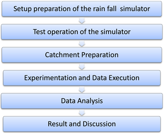
The experimental setups (Simulator) were designed to conduct varying rainfall, micro topography measurements, infiltration measurements and constant drop size vertical distribution in time and space over the catchment constructed. Plots were exposed to simulated rainfall under constant environmental conditions of the study area at 20˚C of room temperature as the simulator is fixed within the laboratory. The setups were designed for small scale runoff measurements, rather than full scale simulation. The setups provide a comparative evaluation of runoff generation, hydrograph, and rainfall runoff correlation graphs peak discharge-time of concentration Nomograms, and time parameters under controlled and documented conditions. Rainfall simulations allow for a wide array of studies to be conducted by varying frequency, intensity, and duration of simulations. Rainfall simulators, unlike natural precipitation events, have the ability to create controlled, reproducible rainfall events. This study utilized rainfall simulation to investigate hill slope runoff generation. The rainfall simulator used to investigate runoff processes is a Fixed but moveable unit so that can be deployed in a variety of settings. The flow diagram of the method used for the study is as below.
2.1. Rainfall Setup and Runoff Collection Procedure
Rainfall Simulator (Basic Hydrology System-S12).
One of the key parameter/variable for the runoff generation, its peak value, time of concentration, ground water table development, and the soil moisture profiles were the rainfall intensity, uniformity, initial condition of the soil and its geometry. It was planned that rainfall simulator available with the Hydraulics Laboratory (HL), Pulchowk Campus, shall be used. After running test experiment with the simulator, two shortcomings were noted. Firstly there was no way to compact the soil used for the development of catchment area at some standard compaction; secondly, the depth of the test beds was not deep enough to allow the system to reach the long term infiltration rate. As the set is fixed and was not portable for field test so it was decided, to carry out the all type of tests on different soil profiles and land use pattern confined catchment within the simulator itself. To carry out rainfall simulations in the set, work began on the design and fabrication of a rainfall simulator. Key design criteria’s involved were as follows.
2.1.1. Portability
The simulator is not portable so that it could not be transported and all tests would be carried out on the soil profiles within the set for the different test plots inside the laboratory hall. But is moveable, so could be made in different slope settings.
2.1.2. Rainfall Variation
Designed simulator should be able to achieved storm intensities in the range from 3 to 30 l/min. Continuous supply of water was not needed as an input for the designed simulator. A sump tank is capable to store the needed volume of water for rainfall generation but if needed continuous supply system was facilitated.
2.2. Model Description
The catchment basin is represented by, shallow tank made of stove enameled mild steel. The rainfall is provided by the row of spray nozzles above the tank and the run of is led to a measuring system at one end of the apparatus. The sketch enclosed shows the important components of the system.
The water supply to the equipment is provided by the electrical centrifugal pump mounted at the floor level beside the sump tank. The water passes through a strainer and flow meter, which measures the rate of flow, and hence to the three inlet control valves. Two of these valves are for controlling the rate of flow to the basin and the third is for controlling the flow to nozzles. The nozzle control valve should be used for adjusting the rate of flow to the desired quantity and then left undisturbed, and all the other supply valves should be firmly closed. When the basin has been filled with soil, the surface profile for the run-off experiments can be formed with the template provided by drawing it along the instrument rails mounted on the channel walls. These instruments rails should be adjusted to have approximately, 3 cm fall towards the outlet weir.
The runoff leaves the catchment by the outflow weir at the sump end of the apparatus. The metal gauge filing this outlet prevents the soil from being washed from the catchment. Flow measurement is carried out using the graduated measuring channel which should be adjusted to the horizontal position by adjustment of the fitted leveling screws. The water falls from the measuring channel into the sump so completing the cycle.
For the well abstraction experiments the water can be added to the catchment by the spray nozzle or by submerged inlets at either end of the catchment. These are designed to be used together and to do this nozzle control valve should be closed with the inlet control valves adjusted until the required flow is achieved.
The level of points on the phreatic surface or water table can be obtained from the manometer bank beside the catchment tank. Each manometer tube is connected to a pressure tapping point in the base of the catchment tank. Before any water table levels are read, it is important to expel air from the tubes connecting the manometers to the pressure tapping points. Figure 1 shows the set of the simulator with its all components.
This item is a completely self-contained unit and requires only laboratory electrical connections. The equipment is supplied with a number of pre-assembled items, together with minimum quantity of minor items to complete the assembly. The procedures to use follow up as:
![]()
![]()
Figure 1. Basic hydrology system-S12 rainfall simulator (hydraulic laboratory).
1) Situate the Main Frame① in the required location and level the Frame by means of the four adjustable feet located at each of the framework legs.
2) Fit the Sump Tank② to the Main Frame1and connects the Pump③ to the Tank Suction Pipe④.
3) Place the Catchment Basin⑤ on to the Main Frame1 and connect Well Drains⑥ and End Drain⑦ flexible pipe work so that these can be led to the Sump Tank②. (Models of current manufacture are shipped assembled).
4) Assemble the Measuring Channel⑧ to the end of the Main Frame① and level the Channel by means of the “level adjusting screws”.
5) Fit the Surge Tank⑨ to the relevant supports at the end of the Main Frame①. Care should be taken to ensure that, when required, this item is easily removable.
6) Assemble the two Sprinkler Pipe work Support Frames⑩ to each end of the Catchment Basin⑤ and check that the upper faces of these Support Frames⑩ are level in both planes.
7) Fit Sprinkler Pipe work Sub Assembly⑪ to Support Frames⑩ and connects the Flexible Pipe⑫ to main pipe work.
8) Assemble the Scraper Blade Carrier⑬ to the Catchment Basin⑤ side rails.
9) Hang the two plastic curtains to the curtain rail which is pre-assembled to the Sprinkler Pipe work⑩ and ensure that these can be easily moved to provide access to the Catchment Basin⑤.
10) Assemble the Twenty Bank Manometer Board⑭ to the Catchment Basin⑤ and adjust this to a level position.
11) Secure all the inter-connecting flexible pipes from the Manometer Board⑭ to the tapping points and ensure that the correct numbering system is adopted in accordance with that illustrated in the Instruction Manual.
12) Complete the installation by connecting the Control Console to the laboratory electrical supply.
13) Check that the overflow pipes are free and can be operated vertically by hand.
2.2.1. Commissioning
Before the start of the experiment the followings should be tested carefully.
1) Check that the pump motor electrical specification complies with the mains supply.
2) Adjust both side rails to “maximum” slope, set the scraper blade to the “lowest” setting and check that the blade clears the two well drains while the carriage traverses the length of the catchment basin.
3) Fill the sump tank, close all valves, switch on pump and check correct pump rotation.
4) Open both inlet control valves to fill catchment basin and check for leaks.
5) Open well drain control valves and check for leaks.
6) Open sprinkler control valve and ensure that all sprinklers are operating correctly. Check for leaks.
7) Adjust inlet control valves and check function of flow meter.
8) Allow water into the measuring channel and confirm that the flow calibration is identical with that of the flow meter indicator over the full range.
9) Close all valves. Fill the catchment basin with 25 mm depth of water to expel air from the manometer tubes, manipulating tubes to assist this Operation, if required.
The equipment is now ready to be filled with soil for experimental purposes.
2.2.2. Technical Specification of the Model
Tank Dimensions:
Length: 2.2 m
Width: 1 m
Height: 0.2 m
Flow meter range 3 - 30 liters/minute
Requirements:
Electricity supply:
1) 220 volt-240 volt/single phase/50 Hz
2) Hydraulic bench or cold water (3 - 30 liter/minute)
3) Well graded sand, clay, silt and gravel
Catchment Dimensions:
Length: 2.02 m
Width: 1 m
Height: 0.15 m
Total volume of soil: 0.30 m3
2.3. Experiment Soil Profile Preparation
As already stated, different types of surfaces were needed to conduct experiments. Land profile was made of sand (mixed and fine), clay, and silt in the catchment tank of the simulator in slopes of 10˚. Soil collection, gradation was carried out in the different laboratory test set up of the campus itself.
2.3.1. Sand Catchment Preparation
After sieving, the sand in the mixed form from the range of 0.2 to 2 mm and in the fine form of size 0.125 mm was kept in the tank to form the catchment area. It was filled as per the specification of the user manual and marked line within the tank of total area 0.202 m2 and volume of 0.24 m3. As per our requirement, the slope was form 10 degree with the horizontal plane as shown in Figure 2. After the reconnaissance, detailed leveling was done by trial and error method so that accuracy was maintained, as all facilities for controlling, collecting and measure runoff. Time observation was done by stopwatch provided. After the completion of the profile preparation the test were carried out and data recording were done simultaneously. As our main aim was to observe the instantaneous runoff discharge, time of concentration and peak discharge due to the
![]()
Figure 2. Photos (simulated rainfall-runoff test on sand plot).
different rainfall intensities from 3 l/min to 13 l/min was recorded. The manometer readings were observed at the one minute intervals with the help of stopwatch.
2.3.2. Silt Catchment Preparation
After sieving, the silt obtained of the size of size 0.06 mm from the sieve size 300 micron passed was collected and kept in the tank to form the catchment area. It was filled as per the specification of the user manual and marked line within the tank of total area 2.02 m2 and volume of 0.24 m3. As per our requirement, the slope was form 10 degree with the horizontal plane as shown in Figure 3. After the reconnaissance, detailed leveling was done by trial and error method so that accuracy was maintained. As all facilities for controlling, collecting, and runoff reading facilities were already associated became easier to observe, collect and measure runoff. Time observation was done by stopwatch provided. After the completion of the profile preparation the test were carried out and data recording were done simultaneously. As our main aim was to observe the instantaneous runoff discharge, time of concentration and peak discharge due to the different rainfall intensities from 3 l/min to 13 l/min was recorded. The manometer readings were observed at the one minute intervals with the help of stopwatch.
2.3.3. Clay Catchment Preparation
The process began by taking the dimensions to be filled by the clay. After the hydrometer test, the clay transported from the place Panchkhal (very famous place of the Kathmandu valley used for the bricks productions) was placed within the catchment tank and leveled at the slope of 10 degree with the horizontal plane as shown in Figure 4. As all facilities for controlling, collecting, and runoff reading facilities were already associated, became easier to observe, collect and measure runoff. Time observation was done by stopwatch provided. After the completion of the profile preparation the test were carried out and data recording were done simultaneously. As our main aim was to observe the instantaneous runoff discharge, time of concentration and peak discharge due to the different rainfall rate from 3 l/min to 13 l/min were recorded at varying initial moisture content so that the change in parameter mainly on time of construction was observed. The manometer readings were observed at the one minute intervals with the help of stopwatch.
![]()
Figure 3. Photos (simulated rainfall-runoff test on silt plot).
![]()
Figure 4. Photos (simulated rainfall-runoff test).
3. Result and Discussion (Model Performance)
3.1. Rainfall-Runoff Hydrographs
After the soil profile preparation, to execute the data the experimental observations were carried out in controlled way from which the result obtained were as explained below.
For individual soil profile in the order of sand, silt and clay, at wet condition under the same room temperature of 20˚C, the rainfall at the rate of 5 lpm was given and the runoff in lps was recorded at the time internal of one minute with the help of stop watch. The rainfall was given in each soil plot up to the peak discharge were obtained and simultaneous time for peak discharge was recorded that is the time of concentration (Tc) for that given rainfall. For the uniform rainfall of 5 lpm, the comparative hydrograph for each soil profiles are shown in (Figure 5). It was observed that the peak discharge were almost of same value of 0.13 lps at the saturated condition was obtained at which the moisture content by each type of soil was 0.40, 0.45 and 0.49 and the initial moisture content was 0.23, 0.1783 and 0.1587 for sand, silt and clay respectively. But the major variation was observed in time of concentration. From the observation it was 9 minute, 16 minute and 18 minute for clay, silt and sand to reach the peak discharge i.e. steady flow condition obtained.
3.2. Rainfall-Runoff Correlation
The rainfall was given at the rate of 4 lpm to 13 lpm to each soil profile separately. Their peak discharges (Qpeak) were recorded and the time of concentration (Tc) was also observed simultaneously. From the observation the peak discharges were around the same values. However slight variations were observed due to factors limitations. The results (Figures 6-8) show individual results of the observations sets. Their resultant rainfall-runoff relations for the best value of correlations (R) were obtained as:
![]()
Figure 5. Comparison of hydrographs for clay, silt and sand slope.
![]()
Figure 6. Typical rainfall runoff correlation generated on sand profile.
![]()
Figure 7. Typical rainfall runoff correlation generated on sand profile.
![]()
Figure 8. Typical rainfall runoff correlation generated on sand profile.
For sand slope,
(3)
For silt slope,
(4)
For clay slope
(5)
The correlation equation obtained with R value above 90% indicates a best condition of the rainfall runoff simulation over the plot scale experiment for individual soil slope profiles.
3.3. Variation in the Runoff Coefficients
For the computation of the runoff coefficient C, in all cases (soil profiles) for the given rainfall intensity, Rational equations were used. There has been a good deal of variation noted in the values of the runoff coefficients for different surfaces (Tables 1-3, Figure 9) the runoff coefficients arranged in order follows as sand, silts and clay. The runoff coefficients lie in the ranges as reported in the literature (i.e. from 0.05 to 0.95). Tables 1-3 show the individual values of runoff coefficients for individual soil plot and Table 4 shows the computed runoff coefficients and rational value as standard. Figure 9 is the comparative chart of the soil plots obtained which shows that the small rainfall rate of runoff coefficient of clay was less than of silt and sand. But at high intensity rainfall the runoff coefficient of clay was high than of silt and sand. It was so because of the initial antecedence moisture conditions.
From the experimental observations the runoff coefficients were obtained as
![]()
Table 1. Rainfall runoff coefficient measurement for sand slope.
![]()
Table 2. Rainfall runoff coefficient measurement for silt slope.
![]()
Table 3. Rainfall runoff coefficient measurement for clay slope.
![]()
Table 4. Observed runoff coefficients and rational values.
![]()
Figure 9. Comparison of runoff coefficient with rainfall for sand, silt and clay slope.
tabulated below. The values are found in range of minimum and maximum values.
4. Conclusions
On the basis of the observations tests, the results strongly indicate the importance of the hydrological processes (rainfall intensity, rainfall rate, and patterns), surface characteristics (geometry) and the antecedent moisture conditions. The major and significant results obtained from this study are outlined as follows:
· Results showed some correlation between the rainfall intensity and the runoff coefficient.
· Runoff coefficients depend on the type of soil and particles size which influences the peak discharge in a rainfall over a catchment area. The values of coefficients obtained by observed gave good results with the rational values as standard. From the experiment, the maximum rainfall runoff coefficients were obtained as 0.428 - 0.53 for sand soil slope, 0.46 - 0.55 for silt soil slope and 0.42 - 0.51 for clay soil slope under uniform rainfall rate of 4 lpm to 13 lpm in each soil slope.
Acknowledgements
The author is extremely grateful to the open journal of civil engineering and my Institute Eastern region campus, Institute of Engineering, TU.