Development and Investigation of the Program Model of Multichannel Queueing System with Unreliable Recoverable Servers in Matlab Environment ()
1. Introduction
Modern computer and telecommunication systems and networks are complicated complexes of technical means that provide receiving, processing and transmitting of different data with definite quality parameters. They are widely represented in all fields of human life and activities, science and technology. The basis of such systems are computer systems of data receiving, processing and transmission with the use of electric, fiber-optic and radio-channels which as a matter of fact are Multichannel Queueing Systems (QS). At present, the field of above mentioned systems and networks are being considerably transformed due to development of wireless data transfer, data storage and processing (cloud computing), fiber optic technology etc. For further development of modern computer and telecommunication systems, it is needed to create appropriate mathematical and software models for their functioning that at the same time would take into consideration peculiarities appropriate to these systems [1] [2] [3] .
It is known that computer operation and telecommunication systems can be greatly influenced by random factors that affect characteristics of their computer capacity, quality of data transfer etc. Examples of random factors could be artificial and natural noises, different levels of noise in the transmission channel, distance change between mobile transmitters, parallel transmission of high priority information, hardware failure and equipment breakdown, weather effects. Random factors especially have great influence over wireless network that is being developed intensively these days. Keeping in mind influence of random factors on the operation process is of great significance while building the adequate mathematical and simulation models and estimating performance calculations of telecommunication systems [4] [5] [6] .
Mathematical methods of queueing system theory that function in a random environment allow to create adequate stochastic models of modern computer and telecommunication systems that take into consideration influence of random factors. Random environment or random medium means random process with final state of space independent from the system. In the case of fixed state of random medium the system functions as classical queueing system. But system parameters (incoming flow, service time distribution etc.) immediately change with the change of random medium state.
In this article multichannel queueing system is discussed which is according to Kendall’s classification belongs to the type A/B/m/K/M, where A is law of arrivals into the system, B―law of Service of Requirements coming into the service, m―number of parallel-functioning equipment (service channel), K is admissible number of requirements in the system, i.e. total number of requirements waiting in a queue and those being served, and M is the number of loading source. Whereas it is believed that system parameters are constant, but processes in the system are considered from the point of view of reproduction and death theory. The subject matter of the investigation in this article is scalable programming model of system with the simplest Poisson requirements arrivals and Exponential service flow [7] [8] [9] .
The software model is developed on the basis of Kolmogorov’s systems of differential equations with relation to probabilities of system states using similarly-named mnemonic rule. Keeping in mind solving equations of the mentioned system in the given starting conditions aspire to their established values that are called steady-state values of probability states, operation characteristics of the system are estimated on their basis.
2. Statement
In this research, while investigating computer and telecommunication management system presented in the form of queueing system consists of servers m = m1 + m2, where m1 is number of main servers, and m2 is number of standby servers operating in background, partial load mode.
Servers are being affected by refusals distributed according to Poisson law with total failure intensity O = O1 + O2 where O1 is failure intensity of main servers, and O2 is failure intensity of standby servers. It is believed that servers operating in background mode are less affected by failures (O1 > O2).
In the system, the possibility of recovering of servers after failures is presupposed and it is fulfilled according to the demonstrative law with total intensity V = V1 + V2, where V1 is recovery intensity of main servers, and V2 is recovery intensity of standby servers. It is supposed that standby servers would switch over to main mode operation for substituting main servers in case of failures, and servers returning to the system after recovery are also included.
In the above described system, Poisson arrival flow of requirements comes for being served with total intensity М = М1 + М2 where М1 is arrival intensity for main servers, and М2 is arrival intensity for standby servers working in the background mode.
Serving arrival flow of requirements follows Exponential probability distribution law with total intensity L = L1 + L2, where L1 is service intensity by main servers, and L2 is service intensity by standby servers.
It should be taken into consideration that in the system it is presupposed to have queue for arriving requirements coming the moment when all servers are busy serving requirements that have come earlier. Total number of arrivals that have possibility to be simultaneously in the system is limited, and equals to K = K1 + K2 + K0, where K1 is the number of arrivals being served by main servers, K2-is the number of arrivals being in the standby servers, and K0 is the number of arrivals that are in the queue.
For characterizing system states
-probabilistic functions are introduced that characterize transition from one state into another under the influence of flows taking place in the system (requirements arrival flow or queue discipline, failure flow and recoveries etc.) and defined as result of multiplication of probabilities of i-state from which transition to appropriate intensity takes place. A key idea of Mnemonic rule of setting up Kolmogorov’s equations is that derivative of probability of any state equals to total sum of probability flows that transit the system into this state, minus the sum of all probability flows that take out the system from this state. General view equation systems, formed according to this rule, looks like this:
, where
; (1)
where
―transition probabilities between states of system, and
and
―transition intensities between indicated states.
Having applied mnemonic rule to the above described system, in consequence of probabilistic reasoning, the system of differential equations can be written as (2) which determines transition probabilities between its states in the following form (it is widely known in literature):
, (2)
where
is probability of event whereby at the moment of time t in the system, in case of given fixed parameter values m1, m2; K1, K2, K0; L1, L2; M1, M2; O1, O2; V1, V2; there are i-requirements, but ratios in case of unknown functions are three-diagonal matrix with values estimated according the following formulae:
(3)
To solve this system of equation with the help of Metlab medium, function ODE23 is used, presupposed for numeral integration of homogenous differential equation systems (HDE). It is applicable for solving simple differential equations, as well as for modelling complex dynamic systems. As it is known, any system of nonlinear HDE can be presented as system of differential equations of the first order in the explicit form of Cauchy
, where x is vector of state, t is time, f―nonlinear vector-function from disposal variables x,t.
Function [t, X] = ode23 (“
”, t0, tf, x0, tol, trace) integrates system HDE using Runge-Kutta’s method of the second and forth order which have parameters: entry
, that is the name of M-file, in which right parts of system HDE are computed, t0―is the initial value of time, tfinal―is final value of time; x0―vector of initial conditions, tol―given precision (default to ode23, tol = 1.e−3); trace―flag regulating exit middleware results (default to zero that suppresses exit of middleware results); output parameters: t―current time; X―two-dimensional arrays where every column corresponds to one variable.
3. Development of Programming Model
The programming model is built in the form of corresponding functions ММmК. The program presupposes computing ratios of three-diagonal matrix for the differential equation system―A, using appropriate functions Matlab: A = full (gallery('tridiag', n, a, b, c)), where a, b, c represent diagonal elements of matrix A.
function MMmK;
clc, close
%%Initial system parameters
DialogM = inputdlg ({'Number of main servers in the system (m1)'
'Number of secondary servers in the system (m2)'
'Number of seats in the queue for requirements (K0)'
'The maximum number of requirements that are on maintenance on the main servers (K1)'
'The maximum number of requirements that are on maintenance on secondary servers (K2)'
'Intensity of exponential maintenance on the main servers (L1)'
'Intensity of exponential maintenance on secondary servers (L2)'
'The intensity of the Poisson input stream of requirements on the main servers (M1)'
'The intensity of the Poisson input stream of requirements on the secondary servers (M2)'
'The intensity of the Poisson failure flow of the main servers (O1)'
'The intensity of the Poisson failure flow of the secondary servers (O2)'
'The intensity of the exponential recovery flow of the main servers (V1)'
'The intensity of the exponential recovery flow of the secondary servers (V2)'}),
'Enter the initial system parameters';
m1=str2double (Dialog M {1}); % Number of main servers in the system
m2=str2double (Dialog M {2}); % Number of secondary servers in the system
K0=str2double (Dialog M {3}); % Number of seats in the queue for requirements
K1=str2double (Dialog M {4}); % The maximum number of requirements that are on maintenance on the main servers
K2=str2double (Dialog M {5}); % The maximum number of requirements that are on maintenance on secondary servers
L1=str2double (Dialog M {6}); %intensity of exponential maintenance on the main servers
L2=str2double (Dialog M {7}); %intensity of exponential maintenance on secondary servers
M1=str2double (Dialog M {8}); %The intensity of the Poisson input stream of requirements on the main servers
M2=str2double (DialogM{9}); %The intensity of the Poisson input stream of requirements on the secondary servers
O1=str2double (Dialog M{10}); %The intensity of the Poisson failure flow of the main servers
O2=str2double (Dialog M{11}); %The intensity of the Poisson failure flow of the secondary servers
V1=str2double (Dialog M{12}); %The intensity of the exponential recovery flow of the main servers
V2=str2double (Dialog M{13}); %The intensity of the exponential recovery flow of the secondary servers
global A
syms n k a b c L N O V K M m m1 m2 M M1 M2 L L1 L2 O O1 O2 V V1 V2 K K0 K1 K2 t T P
L=L1+L2 % The total intensity of exponential flow of service of requirements on the servers of the system
M=M1+M2 % The total intensity of the Poisson flow of incoming requirements
O=O1+O2 %The total intensity of the Poisson flow of failures of servers
V=V1+V2 %The total intensity of the exponential flow of recovery of servers
K=K1+K2+K0;
for i=1:K
a= i *L;
b=-(a+(i -1)*(M-O-V));
c= i *M;
A=full(gallery ('tridiag',K,a,b,c,'double'));
%% Numerical solution of differential equations
P0 = [1;zeros(length(A)-1,1)];
T = [0,0.01];
[t,P] = ode23(@ cmo, T, P0);
End
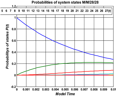
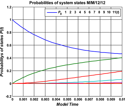
%% Constructing of diagrams of states probabilities
line (t,P,'linew',2)
line (t,P(:,K),'linew',2, 'color','r') %% P(K-1)
grid on
N = length(A)-1;
arr = [0:N]';
str = num2str(arr);
legend (strcat('\bf\itP\rm\bf_', str, '(\itt\rm\bf)'));
title(sprintf('%s Probabilitys of system states M/M/%d/%d', '\bf\fontsize{12}',i, K));
xlabel('\bf\it\fontsize{12} Model Time ')
ylabel('\bf\fontsize{12}\itProbabilitys of states P\rm\bf(\itt\rm\bf)');
set(gca, 'fontweight','bold', 'fontsize',10)
fprintf('\n Stationary probabilities:\n');
for J = 1 : length(A)
fprintf ('\tP%d = %f\n', J-1, P(end,J));
end
fprintf ('\n\t Operational characteristics:\n');
Pnot = P(end,end);
fprintf ('Probabilities of failures Pnot = %f\n', P(end,end));
Q = 1 - Pnot;
Fprintf ('Relative throughput Q = %f\n', Q);
Ab = L*Q;
fprintf ('Absolute throughput Ab = %f\n', Ab);
Pq = sum(P(end, i+1:end));
Fprintf ('Queue length probability Pq = %f\n', Pq);
Ps = sum (P(end, i:end));
Fprintf (' The probability of all servers being busy Ps = %f\n', Ps);
Ns = [0:length(A)-1]*P(end,:)';
fprintf('The average number of requirements in the system Ns = %f\n', Ns);
fprintf('Average time of location of requirements in the system Ts = %f\n', Ns/L);
Nq = [0:(K-i)]*P(end,i:K)';
fprintf('Average queue length Nq = %f\n', Nq);
fprintf('Average time of location of requirements in the queue Tq = %f\n', Nq/L);
function f = cmo(t,P);
%% Functions describing the right-hand sides of differential equations
global A
f = A*P
%Results of program execution
%Stationary probabilities
%The diagram of states probabilities of the system


4. Conclusion
Bearing in mind the significance of computer modelling of complex computer and telecommunication systems presented in the form of QS, in the proposed work, on the basis of Markovian processes of birth and death, scalable program model of QS has been developed with limited number of requirements in the system that allows to determine some probabilistic characteristics of processes happening in them. Program model is created in the Matlab environment that allows graphic presentation of the results. Practical implementation of similar models is highly demanded. Such models significantly simplify researching of queueing systems, they give clear comprehension of states of considered systems, allow to optimize their work.