Stochastic Modelling on Dynamics of Portfolio Diversifications among the Fixed and Operational Investments through Internal Bivariate Linear Birth, Death and Migration Processes

Tirupathi Rao Padi, Chiranjeevi Gudala

Department of Statistics, Pondicherry University, Puducherry, India.

DOI: 10.4236/am.2017.88091                

Abstract

In this paper, a bivariate stochastic process with Poisson postulates has been considered to model the incomings, outgoings and mutual transfers of investments between and within the portfolios during an epoch of time “t”. Stochastic differential equations were obtained from the simple differential difference equations during the epoch of time “Δt”. The notion of bivariate linear birth, death and migration process has been utilized for measuring various statistical characteristics among the investments of Long and Short terms. All possible fluctuations in the investment flow have been considered to explore more meaningful assumptions with contemporary marketing environments. Mathematical relations for proposed statistical measures such as average sizes and variances of short term and long-term investments along with the correlation coefficient between them are derived after obtaining the related differential equations. Numerical illustrations were provided for better understanding of the developed models with practitioner’s point of view.

Keywords

Stochastic Modelling, Portfolio Diversification, Difference-Differential Equations

1. Introduction

Portfolio management has good attraction of researchers of decision making model developments with stochasticity. Formulation of suitable relationship between variables in finance sector and risk assessment is the potential area of application of stochastic modelling as the derivatives of finance investments follow various stochastic processes. Understanding the dynamics of cash flow within one format of investments and also in between two or more formats of investments is possible by measuring the processes in small interval of time so as the behaviour of the investment growth/loss/transformation can be estimated in a epoch of time “t”. A continuous time diffusion process is the suitable option for diversification, growth, and real interest rates among the countries with closed economy and technological uncertainties.

The pioneering activity on modelling of time series data using Brownian motion was initiated in lateral period of 19^th century [1] . Consequently, Bachelier developed theory to study the risk asset prices with Brownian motion using the assumptions of increments of stock prices shall be independent and normally distributed and applied for Paris stock market [2] . Another significant development in this direction is that Construction of Markov processes with continuous through Kolmogorov’s analytic theory [3] .

Bachelier’s model was failed due to the reason that it has not ensured about the stock prices would always be positive though the Geometric Brownian Motion has overcome this drawback [4] . It is evident that Geometric Brownian Motion is a suitable and competent model for stock price movements [5] . The Martingale Approach is used explicitly instead of the classical approach based on partial differential equations for modelling the stock prices. The shift of partial differential equations under boundary conditions to martingale methods has taken long time and which is an essential condition for Feynman-Kac method is, however, that the underlying security processes have to be Markovian diffusions [6] . A constructive approach to stochastic integration with respect to continuous, vector-valued martingales with “continuous” filtrations is presented by Walter Willinger et al. Here the Riemann-Stieltjes approximation is used to discretize time and to carefully discretize the probability space so that almost-sure (path wise) convergence of “simple” Riemann-Stieltjes sums can be established. They have also applied path wise stochastic integration to the theory of security markets with continuous trading [5] . Many theories have been developed to deal with the analysis of stochastic models for the buying and selling of portfolios of securities in continuous time. Another vital finding is Lower tail dependence which contains significant facts for risk-averse investors and is appropriate for portfolio choice, and this a measure of the probability that whether a portfolio will suffer large losses [5] [7] .

Investors can formulate a probability distribution of the probable rates of return on investments to study the likelihood of default and bankruptcy risk [8] . International risk-sharing can yield substantial welfare gains through its effect on expected consumption growth under the assumption that the countries initially hold no riskless assets and asset returns are symmetrically distributed [9] . PDE methods of Kolmogorov and Feller used to study Markov processes with analytic approach and Stochastic Differentials of Itô with probabilistic approach [10] .

The objective of portfolio manager is to minimize the tracking error variance (TEC) for a given projected gain more than the bench marking targets so as the achievement in the wealth of maximum shareholders [11] .

The perception of tail dependence derives from Extreme Value Theory (EVT) allows to designate the tail behaviour of a random variable deprived of postulating its underlying distribution [12] . The risk and returns of investment portfolio in hypothetical scenario based on Heston models have good agreement with practical data pertaining to investigate changing aspects of stock price in real financial markets [13] . A portfolio manager shall have pre-set of information about security returns, developed obvious solutions for the ideal dynamic portfolios with a range of probable constraints. He/she may monitor by using conditioning information to form portfolios that optimize unrestricted performance methods and unconditional tracking efficiency [14] . A unified structure to model and to make evaluation on comparatively large dependence matrices by means of pair vine copula and lowest risk optimal portfolios with respect to five risk measures viz., variance, MAD, minimax, the conditional Value-at-Risk and the conditional Drawdown-at-Risk, has been proposed [15] .

Value at Risk (VaR) is an unsuccessful measure to vigilant the instability on the perspective as it is not using Non-standard Monte Carlo simulations. The magnitude of fat a lower tail, in special circumstances like turbulent markets, general Monte Carlo analysis might not reflect. Then the bi-modal switching structure between assumed normal periods and possible turbulent economic periods may help to resolve the problem [16] . A bivariate stochastic model for Portfolio Management to find the share allocations in Risky and Non-Risky Portfolios of an investment business was developed by considering the linear birth, death and migration processes. It will assess the prevalence of investment inflows from risky to safety assets and vice versa in a portfolio management through the mechanism of growth/loss/and transition processes within a single scheme of investments [17] .

Management of single portfolio consisting of bivariate inflow among the same scheme of the investments such as short term and long-term investments is modelled. However, in practice there will be more than one scheme of investments in which the investors prefer to share their capital. The optimal finance management always suggests the operation of more than one scheme of investments to achieve the objectives like risk minimization, profit maximization, consistency in growth of investment, etc. In order to reach the said goals, this study has proposed a stochastic model with bivariate linear growth and loss processes in two dimensional complementary schemes of investments. Text styles are provided. The formatter will need to create these components, incorporating the applicable criteria that follow.

2. Stochastic Model

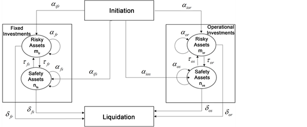
As per this model, there will be two simultaneous operating investment schemes namely long term (fixed) investment and short term (operational) investment. There are two types of complementary growth portfolios namely risky assets and safety assets, operates within each of the fixed and operational investments. Hence this study describes and developed a stochastic model with Bivariate Poisson linear growth and loss processes with two-dimensional investment schemes. The proposed process has the combination of four possible investments such as (i) Fixed Investments with Risky Assets, (ii) Fixed Investments with Safety Assets, (iii) Operational Investments with Risky Assets and (iv) Operational Investments with Safety Assets. Two schemes of investments are connected by a linear combination for getting the joint effect of the total investment policy.

This study has addressed a two-dimensional investment stochastic model with bivariate risk management and portfolio diversification within each dimension. The activities like bonus shares, liquidation, transfer of investments from risky assets to safety assets and vice-versa are expressed with the combination of fixed and operational investments. Each bivariate process is influenced with initial fixed investments in risky and safety assets; as well as initial operational investments in risky and safety assets.

Usually, the objective of Portfolio diversification is to minimize the risk in the investments. However, continuous diversification without any absence makes some times the Portfolio is towards for loss in the long run. The logic of jointing the total effect of portfolio diversification with fixed investment and operational investment through a linear combination of binary variables is considered in this study. Further, it is assumed that the Poisson processes of diversification during the fixed investment and operational investment are complementary. However, the model development is designed to study the factors on growth, evolutions and stipulations and loss processes as an overall phenomenon by combining the conditions of risky and safety assets.

2.1. Notation and Assumptions

Events will be occurred in non-overlapping intervals of time and are statistically independent. a, b, c, d, e, f, g and h be binary constants such that a, b, c, d, e, f, g, h = (0, 1). The notations to use in the formulation are as follows.

i. m_fr: fixed investments in risky assets

ii. m_or: operational investments in risky assets

iii. n_fs: fixed investments in safety assets

iv. n_os: operational investments in safety assets

v. α_ifr: Growth Rate of initial fixed investments in risky assets per unit time

vi. α_ifs: Growth Rate of initial fixed investments in safety assets per unit time

vii. α_ior: Growth Rate of initial operational investments in risky assets per unit time

viii. α_ios: Growth Rate of initial operational investments in safety assets per unit time

ix. α_fr: Growth Rate of fixed investments in risky assets per unit time from the existing m_fr

x. α_fs: Growth Rate of fixed investments in safety assets per unit time from the existing n_fs

xi. α_or: Growth Rate of operational investments in risky assets per unit time from the existing operational investments in risky assets

xii. α_os: Growth Rate of operational investments in safety assets per unit time from the existing operational investments in safety assets

xiii. δ_or: Loss Rate of operational investments in risky assets per unit time from the existing operational investments in risky assets

xiv. δ_os: Loss Rate of operational investments in safety assets per unit time from the existing operational investments in safety assets

xv. δ_fr: Loss Rate of fixed investments in risky assets per unit time from the existing fixed investments in risky assets

xvi. δ_fs: Loss Rate of fixed investments in safety assets per unit time from the existing fixed investments in safety assets

xvii. τ_or: Transition Rate of operational investments from risky assets to safety assets per unit time from the existing operational investments in risky assets

xviii. τ_os: Transition Rate of operational investments from safety assets to risky assets per unit time from the existing operational investments in safety assets

xix. τ_fr: Transition Rate of fixed investments from risky assets to safety assets per unit time from the existing fixed investments in risky assets

xx. τ_fs: Transition Rate of fixed investments from safety assets to risky assets per unit time from the existing fixed investments in safety assets

2.2. Schematic Diagram for the Portfolio Diversification

2.3. Postulates of the Model

i) arrival of a share to the group of Risky Assets during $\Delta t$ through immigration from external sources provided there exits “ $l$ ” number of shares at time “t” is $l\left\{a{\alpha }_{ifr}+\left(1-a\right){\alpha }_{ior}\right\}\Delta t+o\left(\Delta t\right)$ ;

ii) arrival of share to the group of Safety Assets during $\Delta t$ through immigration from external sources provided there exits “ $l$ ” number of shares at time “t” is $l\left\{b{\alpha }_{ifs}+\left(1-b\right){\alpha }_{ios}\right\}\Delta t+o\left(\Delta t\right)$ ;

iii) growth in investment within the group of Risky Assets, during $\Delta t$ provided there exits “m_fr” number of shares in fixed investments and “m_or” number of shares in operational investments already in the said group at time “t” is $\left\{c{m}_{fr}{\alpha }_{fr}+\left(1-c\right)m_{or}{\alpha }_{or}\right\}\Delta t+o\left(\Delta t\right)$ ;

iv) growth in investment within the group of Safety Assets, during $\Delta t$ provided there exits “n_fs” number of shares in fixed investments and “n_os” number of shares in operational investments already in the said group at time “t” is $\left\{d{n}_{fs}{\alpha }_{fs}+\left(1-d\right)n_{os}{\alpha }_{os}\right\}\Delta t+o\left(\Delta t\right)$ ;

v) Transition of share from the group of Risky Assets to the group of Safety Assets during $\Delta t$ provided there exits “m_fr” number of shares in fixed investments and “m_or” number of shares in operational investments are in the Risky Assets group at time “t” is $\left\{e{m}_{fr}{\tau }_{fr}+\left(1-e\right)m_{or}{\tau }_{or}\right\}\Delta t+o\left(\Delta t\right)$ ;

vi) Transition of share from the group of Safety Assets to the group Risky Assets of during $\Delta t$ provided there exits “n_fs” number of shares in fixed investments and “n_os” number of shares in operational investments in Safety Assets group at time “t” is $\left\{f{n}_{fs}{\tau }_{fs}+\left(1-f\right)n_{os}{\tau }_{os}\right\}\Delta t+o\left(\Delta t\right)$ ;

vii) Withdrawal of share (Liquidation) from the group of Risky Assets during $\Delta t$ provided there exits “m_fr” number of shares in fixed investments and “m_or” number of shares in operational investments in the said group at time “t” is $\left\{g{m}_{fr}{\delta }_{fr}+\left(1-g\right)m_{or}{\delta }_{or}\right\}\Delta t+o\left(\Delta t\right)$ ;

viii) Withdrawal of share (Liquidation) from the group of Safety Assets during $\Delta t$ provided there exits “n_fs” number of shares in fixed investments and “n_os” number of shares in operational investments in the said group at time “t” is $\left\{h{n}_{fs}{\delta }_{fs}+\left(1-h\right)n_{os}{\delta }_{os}\right\}\Delta t+o\left(\Delta t\right)$ ;

ix) No growth in number of shares to the groups of Risky Assets and Safety Assets from external sources, no growth in investment within the group of Risky Assets and Safety Assets, no transformation of shares one group to the other group, no withdrawal of shares from the groups of Risky Assets and Safety Assets during an infinitesimal interval of time $\Delta t$ is

$\begin{array}{l}1-\{l\left[\left(a{\alpha }_{ifr}+\left(1-a\right){\alpha }_{ior}\right)+\left(b{\alpha }_{ifs}+\left(1-b\right){\alpha }_{ios}\right)\right]+m_{fr}\left(c{\alpha }_{fr}+e{\tau }_{fr}+g{\delta }_{fr}\right)\\ +m_{or}\left[\left(1-c\right){\alpha }_{or}+\left(1-e\right){\tau }_{or}+\left(1-g\right){\delta }_{or}\right]+n_{fs}\left(d{\alpha }_{fs}+f{\tau }_{fs}+h{\delta }_{fs}\right)\\ +n_{os}\left[\left(1-d\right){\alpha }_{os}+\left(1-f\right){\tau }_{os}+\left(1-h\right){\delta }_{os}\right]\}\cdot \Delta t+O\left(\Delta t\right)\end{array}$

x) Occurrence of other than the above events during an infinitesimal interval of time $\Delta t$ is $O{\left(\Delta t\right)}^2$ .

2.4. Differential Equations of the Model

Let P_m,n(t) be the probability that there exists “m” shares in Risky Assets group and “n” shares in Safety Assets at time “t”. Further let $P_{m,n}\left(t+\Delta t\right)$ be the probability that there exists “m” shares in Risky Assets group and “n” shares in Safety Assets at time “t + Δt”, it may happened as the processes of

$\begin{array}{c}{p}_{m,n}\left(t+\Delta t\right)=p_{m,n}\left(t\right)p_{0,0}\left(\Delta t\right)+p_{m,n-1}\left(t\right)p_{0,1}\left(\Delta t\right)+p_{m-1,n}\left(t\right)p_{1,0}\left(\Delta t\right)\\ +p_{m,n+1}\left(t\right)p_{0,-1}\left(\Delta t\right)+p_{m+1,n}\left(t\right)p_{-1,0}\left(\Delta t\right)+p_{m+1,n-1}\left(t\right)p_{-1,+1}\left(\Delta t\right)\\ +p_{m-1,n+1}\left(t\right)p_{+1,-1}\left(\Delta t\right)+o{\left(\Delta t\right)}^2\end{array}$

$\begin{array}{l}{P^{\prime }}_{m,n}=-\{l\left[\left(a{\alpha }_{ifr}+\left(1-a\right){\alpha }_{ior}\right)+\left(b{\alpha }_{ifs}+\left(1-b\right){\alpha }_{ios}\right)\right]\\ +m\left[\left(c{\alpha }_{fr}+\left(1-c\right){\alpha }_{or}\right)+\left(e{\tau }_{fr}+\left(1-e\right){\tau }_{or}\right)+\left(g{\delta }_{fr}+\left(1-g\right){\delta }_{or}\right)\right]\\ +n\left[\left(d{\alpha }_{fs}+\left(1-d\right){\alpha }_{os}\right)+\left(f{\tau }_{fs}+\left(1-f\right){\tau }_{os}\right)+\left(h{\delta }_{fs}+\left(1-h\right){\delta }_{os}\right)\right]\}{P}_{m,n}\left(t\right)\\ +\left[l\left(b{\alpha }_{ifs}+\left(1-b\right){\alpha }_{ios}\right)+\left(n-1\right)\left(d{\alpha }_{fs}+\left(1-d\right){\alpha }_{os}\right)\right]P_{m,n-1}\left(t\right)\\ +\left[l\left(a{\alpha }_{ifr}+\left(1-a\right){\alpha }_{ior}\right)+\left(m-1\right)\left(c{\alpha }_{fr}+\left(1-c\right){\alpha }_{or}\right)\right]P_{m-1,n}\left(t\right)\\ +\left[\left(n+1\right)\left(h{\delta }_{fs}+\left(1-h\right){\delta }_{os}\right)\right]P_{m,n+1}\left(t\right)+\left[\left(m+1\right)\left(g{\delta }_{fr}+\left(1-g\right){\delta }_{or}\right)\right]P_{m+1,n}\left(t\right)\\ +\left[\left(n+1\right)\left(f{\tau }_{fs}+\left(1-f\right){\tau }_{os}\right)\right]P_{m-1,n+1}\left(t\right)\\ +\left[\left(m+1\right)\left(e{\tau }_{fr}+\left(1-e\right){\tau }_{or}\right)\right]P_{m+1,n-1}\left(t\right);\text{for}m,n\ge 1\end{array}$ (2.4.1)

$\begin{array}{c}{P^{\prime }}_{0,0}\left(t\right)=-\left\{l\left[\left(a{\alpha }_{ifr}+\left(1-a\right){\alpha }_{ior}\right)+\left(b{\alpha }_{ifs}+\left(1-b\right){\alpha }_{ios}\right)\right]\right\}{P}_{0,0}\left(t\right)\\ +\left(h{\delta }_{fs}+\left(1-h\right){\delta }_{os}\right)\cdot P_{0,1}\left(t\right)+\left(g{\delta }_{fr}+\left(1-g\right){\delta }_{or}\right)\cdot P_{1,0}\left(t\right)\end{array}$ (2.4.2)

$\begin{array}{c}{P^{\prime }}_{1,0}\left(t\right)=-\{l\left[\left(a{\alpha }_{ifr}+\left(1-a\right){\alpha }_{ior}\right)+\left(b{\alpha }_{ifs}+\left(1-b\right){\alpha }_{ios}\right)\right]\\ +\left[\left(c{\alpha }_{fr}+\left(1-c\right){\alpha }_{or}\right)+\left(e{\tau }_{fr}+\left(1-e\right){\tau }_{or}\right)+\left(g{\delta }_{fr}+\left(1-g\right){\delta }_{or}\right)\right]\}{P}_{1,0}\left(t\right)\\ +\left(h{\delta }_{fs}+\left(1-h\right){\delta }_{os}\right)P_{1,1}\left(t\right)+\left(g{\delta }_{fr}+\left(1-g\right){\delta }_{or}\right)P_{2,0}\left(t\right)\\ +\left(f{\tau }_{fs}+\left(1-f\right){\tau }_{os}\right)P_{0,1}\left(t\right)\end{array}$ (2.4.3)

$\begin{array}{c}{P^{\prime }}_{0,1}\left(t\right)=-\{l\left[\left(a{\alpha }_{ifr}+\left(1-a\right){\alpha }_{ior}\right)+\left(b{\alpha }_{ifs}+\left(1-b\right){\alpha }_{ios}\right)\right]\\ +\left[\left(d{\alpha }_{fs}+\left(1-d\right){\alpha }_{os}\right)+\left(f{\tau }_{fs}+\left(1-f\right){\tau }_{os}\right)+\left(h{\delta }_{fs}+\left(1-h\right){\delta }_{os}\right)\right]\}{P}_{0,1}\left(t\right)\\ +\left(g{\delta }_{fr}+\left(1-g\right){\delta }_{or}\right)P_{1,1}(t)+\left(e{\tau }_{fr}+\left(1-e\right){\tau }_{or}\right)P_{1,0}\left(t\right)\\ +2\left(h{\delta }_{fs}+\left(1-h\right){\delta }_{os}\right)P_{0,2}\left(t\right)\end{array}$ (2.4.4)

With the initial condition

$P_{M_o}{}_{N_o}\left(t\right)=1,P_{i,j}\left(0\right)=0,\forall i\ne M_o,j\ne N_o$ Where $M_o$ Risky shares and $N_o$ Safety Shares in the Portfolio.

Let $P\left(x,y;t\right)$ be the joint probability generating function of $P_m{}_{,n}\left(t\right)$ ;

where $P\left(x,y;t\right)={\displaystyle \underset{m=0}{\overset{\infty }{\sum }}{\displaystyle \underset{n=0}{\overset{\infty }{\sum }}{x}^m{y}^n{P}_{m,n}\left(t\right)}}$

Multiplying the Equations (2.4.1)-(2.4.4) with $x^m{y}^n$ and summing overall m and n, we obtain

$\begin{array}{l}{\displaystyle \underset{m=0}{\overset{\infty }{\sum }}{\displaystyle \underset{n=0}{\overset{\infty }{\sum }}{x}^m}}{y}^n{P^{\prime }}_{m,n}\left(t\right)\\ ={\displaystyle \underset{m=0}{\overset{\infty }{\sum }}{\displaystyle \underset{n=0}{\overset{\infty }{\sum }}-\left[l\left(\left\{a{\alpha }_{ifr}+\left(1-a\right){\alpha }_{ior}\right\}+\left\{b{\alpha }_{ifs}+\left(1-b\right){\alpha }_{ios}\right\}\right)\right]x^m{y}^n{P}_{m,n}\left(t\right)}}\\ +{\displaystyle \underset{m=0}{\overset{\infty }{\sum }}{\displaystyle \underset{n=0}{\overset{\infty }{\sum }}-\left[m\left(\left\{c{\alpha }_{fr}+\left(1-c\right){\alpha }_{or}\right\}+\left\{e{\tau }_{fr}+\left(1-e\right){\tau }_{or}\right\}+\left\{g{\delta }_{fr}+\left(1-g\right){\delta }_{or}\right\}\right)\right]x^m{y}^n{P}_{m,n}\left(t\right)}}\\ +{\displaystyle \underset{m=0}{\overset{\infty }{\sum }}{\displaystyle \underset{n=0}{\overset{\infty }{\sum }}-\left[n(\{d{\alpha }_{fs}+(1-d){\alpha }_{os}\}+\left\{f{\tau }_{fs}+\left(1-f\right){\tau }_{os}\right\}+\{h{\delta }_{fs}+(1-h){\delta }_{os}\})\right]x^m{y}^n{P}_{m,n}\left(t\right)}}\\ +{\displaystyle \underset{m=0}{\overset{\infty }{\sum }}{\displaystyle \underset{n=0}{\overset{\infty }{\sum }}\left[l\left\{b{\alpha }_{ifs}+\left(1-b\right){\alpha }_{ios}\right\}+\left(n-1\right)\left\{d{\alpha }_{fs}+\left(1-d\right){\alpha }_{os}\right\}\right]x^m{y}^n{P}_{m,n-1}\left(t\right)}}\\ +{\displaystyle \underset{m=0}{\overset{\infty }{\sum }}{\displaystyle \underset{n=0}{\overset{\infty }{\sum }}\left[l\left\{a{\alpha }_{ifr}+\left(1-a\right){\alpha }_{ior}\right\}+\left(m-1\right)\left\{c{\alpha }_{fr}+\left(1-c\right){\alpha }_{or}\right\}\right]x^m{y}^n{P}_{m-1,n}\left(t\right)}}\\ +{\displaystyle \underset{m=0}{\overset{\infty }{\sum }}{\displaystyle \underset{n=0}{\overset{\infty }{\sum }}\left[\left(n+1\right)\left\{h{\delta }_{fs}+\left(1-h\right){\delta }_{os}\right\}\right]x^m{y}^n{P}_{m,n+1}\left(t\right)}}\\ +{\displaystyle \underset{m=0}{\overset{\infty }{\sum }}{\displaystyle \underset{n=0}{\overset{\infty }{\sum }}\left[\left(m+1\right)\left\{g{\delta }_{fr}+\left(1-g\right){\delta }_{or}\right\}\right]x^m{y}^n{P}_{m+1,n}\left(t\right)}}\\ +{\displaystyle \underset{m=0}{\overset{\infty }{\sum }}{\displaystyle \underset{n=0}{\overset{\infty }{\sum }}\left[\left(n+1\right)\left\{f{\tau }_{fs}+\left(1-f\right){\tau }_{os}\right\}\right]x^m{y}^n{P}_{m-1,n+1}\left(t\right)}}\\ +{\displaystyle \underset{m=0}{\overset{\infty }{\sum }}{\displaystyle \underset{n=0}{\overset{\infty }{\sum }}\left[\left(m+1\right)\left\{e{\tau }_{fr}+\left(1-e\right){\tau }_{or}\right\}\right]x^m{y}^n{P}_{m+1,n-1}\left(t\right)}}\end{array}$

$\begin{array}{c}\frac{\text{d}P\left(x,y;t\right)}{\text{d}t}=[\left\{g{\delta }_{fr}+\left(1-g\right){\delta }_{or}\right\}-(\left\{c{\alpha }_{fr}+\left(1-c\right){\alpha }_{or}\right\}+\left\{e{\tau }_{fr}+\left(1-e\right){\tau }_{or}\right\}\\ +\left\{g{\delta }_{fr}+\left(1-g\right){\delta }_{or}\right\})x+\left\{e{\tau }_{fr}+\left(1-e\right){\tau }_{or}\right\}y+\left\{c{\alpha }_{fr}+\left(1-c\right){\alpha }_{or}\right\}{x}^2]\frac{\partial P}{\partial x}\\ +[\left\{h{\delta }_{fs}+\left(1-h\right){\delta }_{os}\right\}-(\left\{d{\alpha }_{fs}+\left(1-d\right){\alpha }_{os}\right\}+\left\{f{\tau }_{fs}+\left(1-f\right){\tau }_{os}\right\}\\ +\left\{h{\delta }_{fs}+\left(1-h\right){\delta }_{os}\right\})y+\left\{f{\tau }_{fs}+\left(1-f\right){\tau }_{os}\right\}x+\left\{d{\alpha }_{fs}+\left(1-d\right){\alpha }_{os}\right\}{y}^2]\frac{\partial P}{\partial y}\\ +\left[l(\left\{a{\alpha }_{ifr}+\left(1-a\right){\alpha }_{ior}\right\}\left(x-1\right)+l\left\{b{\alpha }_{ifs}+\left(1-b\right){\alpha }_{ios}\right\}\left(y-1\right)\right]P\left(x,y;t\right)\end{array}$

2.5. Statistical Measures through the Model

We can obtain the characteristics of the model by using the joint C.G.F. of $P_{m,n}\left(t\right)$ as below

2.5.1. Expected Number of Risky Shares

$m_{1,0}\left(t\right)=\exp \left[-\left\{g{\delta }_{fr}+\left(1-g\right){\delta }_{or}\right\}-\left\{e{\tau }_{fr}+\left(1-e\right){\tau }_{or}\right\}+\left\{c{\alpha }_{fr}+\left(1-c\right){\alpha }_{or}\right\}t\right]M_o$ (2.5.1)

where N_o is initial number of shares in the Risky Asset group

2.5.2. Expected Number of Safety Shares

$m_{0,1}\left(t\right)=\exp \left\{-\left[h{\delta }_{fs}+\left(1-h\right){\delta }_{os}\right]-\left[f{\tau }_{fs}+\left(1-f\right){\tau }_{os}\right]+\left[d{\alpha }_{fs}+\left(1-d\right){\alpha }_{os}\right]\right\}{N}_o$ (2.5.2)

where M_o is initial number of shares in the Safety group.

2.5.3. Variance of Risky Shares

$\begin{array}{l}{m}_{2,0}\left(t\right)=\left\{g{\delta }_{fr}+\left(1-g\right){\delta }_{or}\right\}+\left\{e{\tau }_{fr}+\left(1-e\right){\tau }_{or}\right\}+\left\{c{\alpha }_{fr}+\left(1-c\right){\alpha }_{or}\right\}\ast M_o\\ \ast \exp \left[-\left\{g{\delta }_{fr}+\left(1-g\right){\delta }_{or}\right\}-\left\{e{\tau }_{fr}+\left(1-e\right){\tau }_{or}\right\}+\left\{c{\alpha }_{fr}+\left(1-c\right){\alpha }_{or}\right\}t\right]\\ ÷\left[-\left(-\left\{g{\delta }_{fr}+\left(1-g\right){\delta }_{or}\right\}-\left\{e{\tau }_{fr}+\left(1-e\right){\tau }_{or}\right\}+\left\{c{\alpha }_{fr}+\left(1-c\right){\alpha }_{or}\right\}\right)\right]\\ +\exp \left[2\left(-\left\{g{\delta }_{fr}+\left(1-g\right){\delta }_{or}\right\}-\left\{e{\tau }_{fr}+\left(1-e\right){\tau }_{or}\right\}+\left\{c{\alpha }_{fr}+\left(1-c\right){\alpha }_{or}\right\}\right)t\right]\end{array}$ (2.5.3)

2.5.4. Variance of Safety Shares

$\begin{array}{l}{m}_{0,2}\left(t\right)=\left[\left\{h{\delta }_{fs}+\left(1-h\right){\delta }_{os}\right\}+\left\{f{\tau }_{fs}+\left(1-f\right){\tau }_{os}\right\}+\left\{d{\alpha }_{fs}+\left(1-d\right){\alpha }_{os}\right\}\right]\ast N_o\\ \ast \exp \left[-\left\{h{\delta }_{fs}+\left(1-h\right){\delta }_{os}\right\}-\left\{f{\tau }_{fs}+\left(1-f\right){\tau }_{os}\right\}+\left\{d{\alpha }_{fs}+\left(1-d\right){\alpha }_{os}\right\}t\right]\\ ÷\left[-\left(-\left\{h{\delta }_{fs}+\left(1-h\right){\delta }_{os}\right\}-\left\{f{\tau }_{fs}+\left(1-f\right){\tau }_{os}\right\}+\left\{d{\alpha }_{fs}+\left(1-d\right){\alpha }_{os}\right\}\right)\right]\\ +\exp \left[2\left(-\left\{h{\delta }_{fs}+\left(1-h\right){\delta }_{os}\right\}-\left\{f{\tau }_{fs}+\left(1-f\right){\tau }_{os}\right\}+\left\{d{\alpha }_{fs}+\left(1-d\right){\alpha }_{os}\right\}\right)t\right]\end{array}$ (2.5.4)

2.5.5. Covariance between Risky Shares and Safety Shares

$\begin{array}{l}{m}_{1,1}\left(t\right)=\exp [-(\left\{g{\delta }_{fr}+\left(1-g\right){\delta }_{or}\right\}+\left\{h{\delta }_{fs}+\left(1-h\right){\delta }_{os}\right\}+\left\{e{\tau }_{fr}+\left(1-e\right){\tau }_{or}\right\}\\ +\left\{f{\tau }_{fs}+\left(1-f\right){\tau }_{os}\right\}-\left\{c{\alpha }_{fr}+\left(1-c\right){\alpha }_{or}\right\}-\left\{d{\alpha }_{fs}+\left(1-d\right){\alpha }_{os}\right\})t]\end{array}$ (2.5.5)

3. Numerical Illustration and Sensitivity Analysis

In order to understand the model behavior on more detailed way, simulated numerical data sets were obtained from Equations (1)-(5). The values of $m_{1,0}\left(t\right),m_{0,1}\left(t\right),m_{2,0}\left(t\right),m_{0,2}\left(t\right)$ and $m_{1,1}\left(t\right)$ are computed for different values of ${\alpha }_{fr},{\alpha }_{or},{\alpha }_{fs},{\alpha }_{os},{\delta }_{fr},{\delta }_{or},{\delta }_{fs},{\delta }_{os},{\tau }_{fr},{\tau }_{or},{\tau }_{fs},{\tau }_{os},N_o,M_o$ and $t$ when the remaining are constant and presented in Table 1 and Table 2.

Table 1. Values of m₁₀, m₀₁,m₂₀, m₀₂, and m₁₁ for varying values of α_fr, α_or, α_fs, α_os, δ_fs, δ_or, δ_fs,δ_os when the remaining are constants.

Table 2. Values of m₁₀, m₀₁, m₂₀, m₀₂, and m₁₁ for varying values of τ_fs, τ_os, τ_fr, τ_or, N₀, M₀ and t when the remaining are constants.

Figures

Figure 1. The changing patterns of statistical measures with respect to the study parameters.

4. Findings

The changing patterns of statistical measures with respect to the study parameters are presented in Table 1 and further they are presented in figures for better understanding of model behaviour with related parameters. The following are some observations.

Figure 1(a) & Figure 1(b) displayed that Mean and Variances of number of Risky Asset’s shares are increasing functions of growth (arrival) rate of Fixed investments and also increased with Operational investments when all other parameters are constants. And Co-variance of number of Risky Asset’s Shares with Safety Asset’s Shares are increasing functions of growth (arrival) rate of Risky Asset’s Shares with Fixed investments and Operational investments, when all other parameters are constant. It is also observed that Expected number of Safety Asset’s Shares and variance of number of Safety Asset’s Shares are invariant of Growth Rate of initial fixed investments in Risky Assets per unit time and Growth Rate of initial operational investments in Risky Assets per unit time.

From Figure 1(c) & Figure 1(d), it is observed that, Average and Variances of Safety Assets are increasing functions of growth (arrival) rate of Fixed investments and also increased with Operational investments when all other parameters are constant. Co-variance of Risky Asset’s Shares with Safety Asset’s Shares are increasing functions of growth (arrival) rate of Safety Assets Shares with Fixed investments and Operational investments, when all other parameters are constant. It is also observed that Expected number of Risky Asset’s Shares and variance of number of Risky Asset’s Shares are invariant of Growth Rate of initial fixed investments in Safety Assets per unit time and Growth Rate of initial operational investments in Safety Assets per unit time.

From Figure 1(e) & Figure 1(f), it is apparent that, Aggregate and Variability of Risky Asset’s Shares are decreasing functions of growth (arrival) rate of Fixed investments and also increased with Operational investments when all other parameters are constant. Co-variance of Risky Asset’s Shares with Safety Asset’s Shares are decreasing functions of loss rate of Risky Asset’s Shares with Fixed investments and Operational investments, when all other parameters are constant. And Expected number of Safety Asset’s Shares and variance of Safety Asset’s Shares are invariant of Loss Rate of fixed investments in Risky Asset’s per unit time from the existing m_fr and Loss Rate of operational investments in Risky Assets per unit time from the existing m_or.

Figure 1(i) & Figure 1(j) exhibited that Mean and Variances Safety Asset’s Shares are decreasing functions of growth (arrival) rate of Fixed investments and also increased with Operational investments when all other parameters are constant. Co-variance of Risky Asset’s Shares with Safety Asset’s Shares are decreasing functions of loss rate of Safety Asset’s Shares with Fixed investments and Operational investments, when all other parameters are constant. Aggregate and variance of Risky Asset’s Shares are invariant of Loss Rate of fixed investments in Safety Assets per unit time from the existing n_fs and Loss Rate of operational investments in Safety Assets per unit time from the existing n_os.

Figure 1(k) & Figure 1(l) show that average number of Risky Asset’s shares and variance of Risky Asset’s Shares are decreasing functions of loss rate of Safety Assets with Fixed investments and Operational investments, when all other parameters are constant. Co-variance of Risky asset’s shares with Safety asset’s shares are decreasing functions of transformation rate of Risky asset’s shares with Fixed investments and Operational investments, when all other parameters are constant. Average and variance of number of Safety asset’s shares are invariant of Transition Rate of operational investments from Risky assets to Safety assets per unit time from the existing m_or and Transition Rate of fixed investments from Risky assets to Safety assets per unit time from the existing m_fr.

Figure 1(m) & Figure 1(n) disclosed that, aggregate and Variances of Safety Asset’s Shares are decreasing functions of loss rate of Safety Asset’s Shares with Fixed investments and Operational investments, when all other parameters are constant. Co-variance of Risky Assets Shares with Safety Assets Shares are decreasing functions of transformation rate of Safety Assets Shares with Fixed investments and Operational investments, when all other parameters are constant. Expectation and variance of number of Risky Asset’s Shares are invariant of Transition Rate of fixed investments from Safety Assets to risky assets per unit time from the existing n_fs and Transition Rate of operational investments from Safety Assets to Risky Assets per unit time from the existing n_os.

Figure 1(o) exhibited that Mean and Variance of Risky Assets Shares are increasing functions of initial size of Risky shares $N_o$ . Whereas, expected number and variance of Safety asset’s shares along with co-variance between Risky asset’s shares and of Safety asset’s shares are invariant with Fixed investments; and Operational investments when all other parameters are constant.

Figure 1(p) displayed that expected number of Safety asset’s shares and variance of Risky asset’s shares are increasing functions of initial size of Safety shares $M_o$ . Whereas, expected number of Risky Asset’s Shares, the variance of Risky Asset’s shares; Co-variance of Risky Asset’s shares with Safety Asset’s shares are invariant with Fixed investments and Operational investments when all other parameters are constant.

Figure 1(q) exhibited that, average number of Risky Asset’s Shares and Safety Asset’s Shares, variance of Risky Asset’s shares and variance of Safety Asset’s shares; Co-variance of Risky Asset’s Shares with Safety Asset’s shares are decreasing functions of time t.

Conflicts of Interest

The authors declare no conflicts of interest.

References

[1]	Thiele, T.N. (1880) Sur la compensation de quelques erreurs quasisystématiques par la méthode des moindres carrés. Reitzel, Copenhagen.
[2]	Bachelier, L. (1900) Théoriedela Spéculation. Annales Scientifiques de l’école Normale Supérieure, 3, 21-86. https://doi.org/10.24033/asens.476
[3]	L′evy, P. (1955) W. Doblin (V. Doeblin) (1915-1940). Revue d’Histoire des Sciences et de leurs Applications, 8, 107-115. |https://doi.org/10.3406/rhs.1955.3509
[4]	Samuelson, P. (1965) Rational Theory of Warrant Pricing. Industrial Management Review, 6, 13-39.
[5]	Jarrow, R. and Protter, P. (2004) A Short History of Stochastic Integration and Mathematical Finance the Early Years, 1880-1970. IMS Lecture Monograph, 45, 1-17. https://doi.org/10.1214/lnms/1196285381
[6]	Harrison, J.M. and Kreps, D.M. (1979) Martingales and Arbitrage in Multiperiod Securities Markets. Journal of Economic Theory, 20, 381-408. https://doi.org/10.1016/0022-0531(79)90043-7
[7]	Harrison, J.M. and Pliska, S.R. (1981) Martingales & Stochastic Integrals in the Theory of Continuous Trading. Stochastic Processes and their Applications, 11, 215-260 https://doi.org/10.1016/0304-4149(81)90026-0
[8]	Francis, J.C. (1986) lnzlestrrrents—Analysis and Management. MCGraw Hill, International Editions.
[9]	Obstfeld, M. (1994) Risk-Taking, Global Diversification, and Growth. The American Economic Review, 84, 1310-1329.
[10]	Doob, J.L. (1996) The Development of Rigor in Mathematical Probability (1900-1950). In: Pier, J.-P., Ed., Development of Mathematics 1900-1950, Birkhauser Verlag AG, Basel. https://doi.org/10.2307/2974673
[11]	Baptista, A.M. (2008) Optimal Delegated Portfolio Management with Background Risk. Journal of Banking & Finance, 32, 977-985. https://doi.org/10.1016/j.jbankfin.2007.07.009
[12]	DiTragliaa, F.J. and Gerlach, J.R. (2013) Portfolio Selection: An Extreme Value Approach. Journal of Banking & Finance, 37, 305-323. https://doi.org/10.1016/j.jbankfin.2012.08.022
[13]	Li, J.-C. and Mei, D.-C. (2014) The Returns and Risks Investment Portfolio in a Financial Market. Physica A, 406, 67-72. https://doi.org/10.1016/j.physa.2014.03.005
[14]	Chiang, I-H.E. (2015) Modern Portfolio Management with Conditioning Information. Journal of Empirical Finance, 33, 114-134. https://doi.org/10.1016/j.jempfin.2015.05.003
[15]	Bekirosa, S., Hernandez, J.A., Hammoudeh, S. and Nguyen, D.K. (2005) Multivariate Dependence Risk and Portfolio Optimization: An Application to Mining Stock Portfolios. Resources Policy, 46, 1-11.
[16]	Karagiannidis, I. and Wilford, D.S. (2015) Modeling Fund and Portfolio Risk: A Bi-Modal Approach to Analyzing Risk in Turbulent Markets. Review of Financial Economics, 25, 19-26. https://doi.org/10.1016/j.rfe.2015.02.005
[17]	Padi, T.R. and Gudala, C. (2015) Linear Birth, Death and Migration Processes for Portfolio Management Modelling. IOSR Journal of Mathematics (IOSR-JM), 11, 29-36.