Boundedness of Fractional Integral with Variable Kernel and Their Commutators on Variable Exponent Herz Spaces ()
Received 25 April 2016; accepted 26 June 2016; published 29 June 2016

1. Introduction
Let ,
, 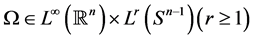 is homogenous of degree zero on
 ,
,  denotes the unit sphere in
 . If
. If
(i) For any , one has
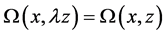 ;
;
(ii) 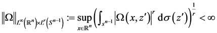
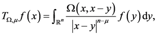
The fractional integral operator with variable kernel  is defined by
The commutators of the fractional integral is defined by
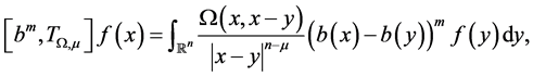
When , the above integral takes the Cauchy principal value. At this time
 ,
,  is much more close related to the elliptic partial equations of the second order with variable coefficients. Now we need the further assumption for
![]() . It satisfies
. It satisfies
![]()
For![]() , we say Kernel function
, we say Kernel function ![]() satisfies the
satisfies the ![]() -Dini condition, if
-Dini condition, if ![]() meets the conditions (i), (ii) and
meets the conditions (i), (ii) and
![]()
where ![]() denotes the integral modulus of continuity of order r of
denotes the integral modulus of continuity of order r of ![]() defined by
defined by
![]()
where ![]() is the a rotation in
is the a rotation in ![]()
![]()
when![]() ,
, ![]() is the fraction integral operator
is the fraction integral operator
![]()
The corresponding fractional maximal operator with variable kernel is defined by
![]()
We can easily find that when ![]()
![]() is just the fractional maximal operator
is just the fractional maximal operator
![]()
Especially, in the case![]() , the fractional maximal operator reduces the Hardy-Littelewood maximal operator.
, the fractional maximal operator reduces the Hardy-Littelewood maximal operator.
Many classical results about the fractional integral operator with variable kernel have been achieved [1] - [5] . In 1971, Muckenhoupt and Wheeden [6] had proved the operator ![]() was bounded from
was bounded from ![]() to
to![]() . In 1991, Kováčik and Rákosník [7] introduced variable exponents Lebesgue and Sobolev spaces as a new method for dealing with nonlinear Dirichet boundary value problem. In the last 20 years, more and more researchers have been interested in the theory of the variable exponent function space and its applications [8] - [14] . In 2012, Wu Huiling and Lan Jiacheng [15] proved the bonudedness property of
. In 1991, Kováčik and Rákosník [7] introduced variable exponents Lebesgue and Sobolev spaces as a new method for dealing with nonlinear Dirichet boundary value problem. In the last 20 years, more and more researchers have been interested in the theory of the variable exponent function space and its applications [8] - [14] . In 2012, Wu Huiling and Lan Jiacheng [15] proved the bonudedness property of ![]() with a rough kernel on variable exponents Lebesgue spaces.
with a rough kernel on variable exponents Lebesgue spaces.
Recently, Wang and Tao [16] introduced the class of Herz spaces with two variable exponents, and also studied the Parameterized Littlewood-Paley operators and their commutators on Herz spaces with variable exponents.
The main purpose of this paper is to discuss the boundedness of the fractional integral with variable kernel
![]() and their commutators
and their commutators ![]() are bonuded on Herz spaces with two variable exponents or not.
are bonuded on Herz spaces with two variable exponents or not.
Throughout this paper ![]() denotes the Lebesgue measure,
denotes the Lebesgue measure, ![]() means he characteristic function of a measurable set
means he characteristic function of a measurable set![]() . C always means a positive constant independent of the main parameters and may change from one occurrence to another.
. C always means a positive constant independent of the main parameters and may change from one occurrence to another.
2. Definition of Function Spaces with Variable Exponent
In this section we define the Lebesgue spaces with variable exponent and Herz spaces with two variable ex- ponent, and also define the mixed Lebesgue sequence spaces.
Let E be a measurable set in ![]() with
with![]() . We first define the Lebesgue spaces with variable exponent.
. We first define the Lebesgue spaces with variable exponent.
Definition 2.1. see [1] Let ![]() be a measurable function. The Lebesgue space with variable
be a measurable function. The Lebesgue space with variable
exponent ![]() is defined by
is defined by
![]()
The space ![]() is defined by
is defined by
![]()
The Lebesgue spaces ![]() is a Banach spaces with the norm defined by
is a Banach spaces with the norm defined by
![]()
We denote
![]()
![]() .
.
Then ![]() consists of all
consists of all ![]() satisfying
satisfying ![]() and
and![]() .
.
Let M be the Hardy-Littlewood maximal operator. We denote ![]() to be the set of all function
to be the set of all function ![]() satisfying the M is bounded on
satisfying the M is bounded on![]() .
.
Definition 2.2. see [17] Let![]() . The mixed Lebesgue sequence space with variable exponent
. The mixed Lebesgue sequence space with variable exponent
![]() is the collection of all sequences
is the collection of all sequences ![]() of the measurable functions on
of the measurable functions on ![]() such that
such that
![]()
![]()
Noticing![]() , we see that
, we see that
![]()
Let ![]()
Definition 2.3. see [16] Let![]() . The homogeneous Herz space with variable ex- ponent
. The homogeneous Herz space with variable ex- ponent ![]() is defined by
is defined by
![]()
where
![]()
Remark 2.1. see [16] (1) If ![]() satisfying
satisfying![]() , then
, then
![]()
(2) If ![]() and
and![]() , then
, then ![]() and
and![]() . Thus, by Lemma 3.7
. Thus, by Lemma 3.7
and Remark 2.2, for any![]() , we have
, we have
![]()
where
![]()
![]()
This implies that![]() .
.
Remark 2.2. Let![]() . then
. then
![]()
where
![]()
Definition 2.4. see [18] For![]() , the Lipschitz space
, the Lipschitz space ![]() is defined by
is defined by
![]() (1.1)
(1.1)
3. Properties of Variable Exponent
In this section we state some properties of variable exponent belonging to the class ![]() and
and![]() .
.
Proposition 3.1. see [1] If ![]() satisfies
satisfies
![]()
![]()
then, we have![]() .
.
Proposition 3.2. see [15] Suppose that![]() ,
,![]() . Let
. Let![]() , and define the variable exponent
, and define the variable exponent ![]() by:
by:![]() . Then we have that for all
. Then we have that for all![]() ,
,
![]()
Proposition 3.3. Suppose that![]() ,
, ![]() ,
, ![]() ,
,![]() . Let
. Let
![]() , and define the variable exponent
, and define the variable exponent ![]() by:
by:![]() . Then
. Then
![]()
Proof
![]()
By Proposition 3.2, we get
![]()
Now, we need recall some lemmas
Lemma 3.1. see [13] Given ![]() have that for all function f and g,
have that for all function f and g,
![]()
Lemma 3.2. see [19] Suppose that![]() ,
, ![]() ,
, ![]() satisfies the
satisfies the ![]() -Dini con- dition. If there exists an
-Dini con- dition. If there exists an ![]() such that
such that ![]() then
then
![]()
Lemma 3.3. see [20] Suppose that![]() , the variable function
, the variable function ![]() is defined by
is defined by![]() ,
,
then for all measurable function f and g, we have
![]()
Lemma 3.4. see [21] Suppose that ![]() and
and![]() .
.
1) For any cube and![]() , all the
, all the![]() , then:
, then: ![]()
2) For any cube and![]() , then
, then ![]() where
where
![]()
Lemma 3.5. see [22] If![]() , then there exist constants
, then there exist constants ![]() such that for all balls B in
such that for all balls B in ![]() and all measurable subset
and all measurable subset ![]()
![]()
Lemma 3.6. see [13] If![]() , there exist a constant
, there exist a constant ![]() such that for any balls B in
such that for any balls B in![]() . we have
. we have
![]()
Lemma 3.7. see [16] Let![]() . If
. If![]() , then
, then
![]()
4. Main Theorems and Their Proof
Theorem 1. Suppose that![]() ,
, ![]() ,
, ![]() ,
,
![]() with
with![]() . And let
. And let ![]() satisfy
satisfy ![]() and define the vari-
and define the vari-
able exponent ![]() by
by![]() . Then the operators
. Then the operators ![]() is bounded from
is bounded from ![]() to
to
![]() .
.
Theorem 2. Let ![]() Suppose that
Suppose that![]() ,
,
![]() ,
, ![]() with
with![]() . If
. If ![]() satisfy
satisfy
![]() and define the variable exponent
and define the variable exponent ![]() by
by![]() . Then the com-
. Then the com-
mutators ![]() is bounded from
is bounded from ![]() to
to![]() .
.
Proof of Theorem1:
Let![]() . We write
. We write
![]()
From definition of ![]()
![]()
Since
![]()
where
![]()
![]()
![]()
And![]() , thus
, thus
![]()
That is
![]()
This implies only to prove![]() . Denote
. Denote ![]()
Now we consider![]() . Applying Lemma 3.7
. Applying Lemma 3.7
![]()
where
![]()
By the Proposition 3.2, we get
![]()
Since![]() , then we have
, then we have![]() , and
, and
![]()
By Lemma 3.7 and Remark 2.2, we get
![]()
Hence![]() , and
, and![]() , this implies that
, this implies that
![]()
Now, we estimate of ![]() using size condition of
using size condition of ![]() and Minkowski inequality, when
and Minkowski inequality, when ![]() we get,
we get,
![]()
Since ![]() we define the variable exponent
we define the variable exponent![]() , by Lemma 3.3 we get
, by Lemma 3.3 we get
![]()
According Lemma 3.4 and the formula![]() , then we have
, then we have
![]() (1.2)
(1.2)
By Lemma 3.2, we get
![]()
It follows that
![]() (1.3)
(1.3)
By the Equation (1.3) and using Lemmas 3.1, 3.5, 3.6, 3.7, we can obtain
![]()
where
![]()
Since![]() , then we have
, then we have![]() , and
, and
![]()
Now if![]() , then we have
, then we have
![]()
where ![]()
If![]() , then we have
, then we have
![]()
where![]() , this implies that
, this implies that
![]()
Finally, we estimate ![]() by Lemma 3.7, we get
by Lemma 3.7, we get
![]() (1.4)
(1.4)
Note that, when![]() ,
, ![]() , then
, then![]() . Therefore, applying the generalized Hölder’s In- equality, we have
. Therefore, applying the generalized Hölder’s In- equality, we have
![]()
Define the variable exponent ![]() by Lemma 3.3, then we have
by Lemma 3.3, then we have
![]()
![]()
According Lemma 3.4 and the formula![]() , we have
, we have ![]() Then we get
Then we get
![]() (1.5)
(1.5)
From Equations (1.4), (1.5) and using Lemma 3.7, and ![]() we can obtain
we can obtain
![]()
Note that
![]() see [9] .
see [9] .
Then we have
![]()
where
![]()
Since ![]() and
and![]() , as the same
, as the same ![]() we have
we have
![]()
This completes the proof Theorem 1.
Proof of Theorem 2
Let![]() ,
,![]() . We write
. We write
![]()
From definition of ![]()
![]()
Since
![]()
where
![]()
![]()
![]()
And![]() . The similar to prove of Theorem 1
. The similar to prove of Theorem 1
![]()
Hence![]() . Denote
. Denote ![]()
First we estimate![]() . Note that
. Note that ![]() is bonuded on
is bonuded on ![]() (Proposition 3.3), similarly to esti-
(Proposition 3.3), similarly to esti-
mate for ![]() in the proof of the Theorem 1, we get that
in the proof of the Theorem 1, we get that
![]()
That is
![]()
Now, we estimate of![]() . Using size condition of
. Using size condition of ![]() and Minkowski inequality, when
and Minkowski inequality, when ![]() we get,
we get,
![]()
We have that
![]() (1.6)
(1.6)
The similar way to estimate of ![]() in the proof of Theorem 1, we get that
in the proof of Theorem 1, we get that
![]() (1.7)
(1.7)
By (1.7) and lemma 3.7, we obtain that
![]()
where
![]()
Since ![]() and
and![]() , the similar way to estimate
, the similar way to estimate ![]() in the proof of Theorem1, we can obtain that
in the proof of Theorem1, we can obtain that
![]()
where![]() , this implies that
, this implies that
![]()
Finally, we estimate![]() . Note that, when
. Note that, when![]() ,
, ![]() , then
, then![]() , we can obtain that
, we can obtain that
![]()
Then we have
![]() (1.8)
(1.8)
Applying the generalized Hölder’s Inequality, we get
![]()
Define the variable exponent ![]() by Lemma 3.3, then we have
by Lemma 3.3, then we have
![]()
According Lemma 3.4 and the formula![]() , we have
, we have![]() . Then we get
. Then we get
![]()
By (1.8), we can obtain that
![]() (1.9)
(1.9)
Then by (1.9) and Lemma 3.7, we have
![]()
where
![]()
Furthermore, when![]() , note that
, note that ![]() see [9] , the similar way to estimate
see [9] , the similar way to estimate![]() , we get
, we get
![]()
We can conclude that
![]()
where![]() , this implies that
, this implies that
![]()
This completes the proof Theorem 2.
Competing Interests
The authors declare that they have no competing interests.
Acknowledgements
This paper is supported by National Natural Foundation of China (Grant No. 11561062).
NOTES
![]()
*Corresponding author.