Boundedness for Commutators of Calderón-Zygmund Operator on Herz-Type Hardy Space with Variable Exponent ()

Abstract

Keywords

Share and Cite:

Received 25 May 2016; accepted 26 June 2016; published 29 June 2016

1. Introduction

In 2012, Hongbin Wang and Zongguang Liu [1] discussed boundedness Calderón-Zygmund operator on Herz- type Hardy space with variable exponent. M. Luzki [2] introduced the Herz space with variable exponent and proved the boundedness of some sublinear operator on these spaces. Li’na Ma, Shuhai Li and Huo Tang [3] proved the boundedness of commutators of a class of generalized Calderón-Zygmund operators on Labesgue space with variable exponent by Lipschitz function. Mitsuo Izuki [4] proved the boundedness of commutators on Herz spaces with variable exponent. Lijuan Wang and S. P. Tao [5] proved the boundedness of Littlewood- Paley operators and their commutators on Herz-Morrey space with variable exponent. In this paper we prove the boundedness of commutators of singular integrals with Lipschitz function or BMO function on Herz-type Hardy space with variable exponent.

In this section, we will recall some definitions.

Definition 1.1. Let T be a singular integral operator which is initially defined on the Schwartz space. Its values are taken in the space of tempered distributions such that for x not in the support of f,

(1.1)

where f is in, the space of compactly bounded function.

Let Here the kernel k is function in away from the diagonal and satisfies the standard estimate

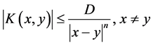(1.2)

and

(1.3)

provided that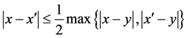

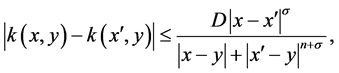(1.4)

provided that such that is called standard kernel and the class of all kernels that

satisfy (1.2), (1.3), (1.4) is denoted by. Let T be as in (1.1) with kernel. If T is bounded from L^p to L^p with, then we say that T is Calderón-Zygmund operator.

Let Ω be a measurable set in with. We first defined Lebesgue spaces with variable exponent.

Definition 1.2. [4] Let be a measurable function. The Lebesgue space with variable exponent is defined by

(1.5)

The space is defined by

The Lebesgue space is a Banach space with the norm defined by

(1.6)

We denote

.

Then consists of all satisfying and.

Let M be the Hardy-Littlewood maximal operator. We denote to be the set of all function satisfying that M is bounded on.

Let

Proposition 1.1. See [1] . If satisfies

(1.7)

(1.8)

then, we have.

Proposition 1.2. [6] Suppose that, if then

(1.9)

for all balls with.

Definition 1.3. [7] Let, and. The homogeneous Herz space with variable exponent is defined by

(1.10)

where

(1.11)

The non-homogeneous Herz space with variable exponent is defined by

(1.12)

where

(1.13)

Definition 1.4. [1] Let, and and. Suppose that is maximal function of f. Homogeneous variable exponent Herz-tybe Hardy spaces is defined by

(1.14)

with norm

(1.15)

Definition 1.5. [1] Let, , and non negative integer

A function g on is said to be a central, if satisfies

1);

2);

3).

What’s more, when,

(1.16)

Definition 1.6. [7] the Lipschiz space is defined by

(1.17)

Definition 1.7. For, the bounded mean oscillation space is defined by

2. Main Result and Proof

In order to prove result, we need recall some lemma.

Lemma 2.1. ( [3] ) Let, T be Calderón-Zygmund operator, ,

Then,

(2.1)

Lemma 2.2. ( [8] ) Let; if and, then

(2.2)

where

Lemma 2.3. ( [2] ) Let. Then for all ball B in,

(2.3)

Lemma 2.4. ( [2] ) Let then for all measurable subsets, and all ball B in

(2.4)

where, are constants with

Lemma 2.5. ( [4] ) Let, and with then

Lemma 2.6. ( [9] ) Let function and T be a Calderón-Zygmund operator. Then

Theorem 2.1. Let, , , , and

where are a constants, then are bounded from to.

Proof: we suffices to prove homogeneous case. Let, in the sense, where each is a central -atom with supp. Write

We have

(2.5)

(2.6)

By virtue of Lemma 2.1, we can easily see that

First we estimate F₁. For each and we shall get

(2.7)

Thus by Lemma 2.3, Lemma 2.4 and Proposition 1.2, we get

(2.8)

When and, by Hölder’s inequality and (2.8), we calculations

(2.9)

where by, we get

(2.10)

Now we estimate F₃. For each, we shall get

(2.11)

Using the Lemma 2.3 and Lemma 2.4 and Proposition 1.2, we obtain

(2.12)

When and, by Hölder’s inequality and (2.12), we have

(2.13)

When by, we have

(2.14)

Combining (2.10)-(2.14), we get

Theorem 2.2. Let, , , and where are a

constants, then are bounded from to.

Proof: we suffices to prove homogeneous case. Let, in the sense, where each is a central -atom with supp. Write

We have

By inequality (2.5)we have

Firstly we estimate F₂ by Lemma 2.6 we can see

Now we consider the estimates of F₁. Note that for each, , and, by generalized Hölder’s inequality and Lemma 2.2, we have

Thus by Lemma 2.5 we get

(2.16)

Thus by Lemma 2.3, Lemma 2.4 and noting that we get

(2.17)

When and, by Hölder’s inequality and (2.17), we calculations

(2.18)

when by, we get

(2.19)

Finally we consider the estimates of F₃. Note that for each, , and, by generalized Hölder’s inequality and Lemma 2.2. we have

(2.20)

Thus by Proposition 1.2, and Lemma 2.5, we get

(2.21)

Thus by Lemma 2.3, Lemma 2.4 and noting that we get

(2.22)

When and, by Hölder’s inequality and (2.22),we calculations

(2.23)

when by, we get

(2.24)

combining (2.14)-(2.24) the prove is completed.

Acknowledgements

This paper is supported by National Natural Foundation of China (Grant No. 11561062).

NOTES

^*Corresponding author.

Conflicts of Interest

The authors declare no conflicts of interest.

References