Development of an Aggregate Air Quality Index Using a PCA-Based Method: A Case Study of the US Transportation Sector ()
1. Introduction
Transport modes emit air pollutants such as carbon monoxide (CO), nitrogen oxides (NOx), particulate matter (PM), sulfur dioxide (SO2), and volatile organic compounds (VOCs) into the air through fossil fuel combustion. Such air pollution frequently exposes human health to acute and chronic diseases, and in the short- and long- terms might result in premature death and declines in life expectancy [1] . Further, it is reported by several researchers that outdoor air pollution negatively affects the productivity of indoor workers [2] - [7] .
Transportation is essential for economic growth at the local and national levels, but it is highly connected to environmental pollution, especially air pollution [8] . Gorham’s 2002 report [9] for the United Nations shows how much fossil fuel is being combusted by transportation: the transportation sector consumes 25 percent of total worldwide energy consumption and uses more than 50 percent of the total oil produced. Furthermore, annual demand for transport modes is projected to grow by 3.6 percent in developing countries and by 1.5 percent in developed countries [9] . Finally, it might be appropriate to recognize transportation’s air pollution emissions as one of the most serious sources of ongoing atmospheric pollution in the world.
Daily air quality indices that evaluate the levels of air pollutants measured at monitoring stations have been developed by a number of researchers [10] - [22] to inform the public about how polluted their living areas are. However, the indices developed until now have a couple of limitations. First, mathematical models for developing air quality indices are based on daily air pollution data (to report daily levels of health concern to the public); this means that without any data measured per day, the model is useless. Second, air pollution data measured at monitoring stations generally represent the levels of overall air pollution in that area, and thus the model cannot be applied to any specific air emissions source, e.g., transportation, to suggest the degree of pollution by transport mode in a state or city.
Nonetheless, under the Clean Air Act1 the US Environmental Protection Agency (USEPA) has an obligation to provide national emissions inventory (NEI) data2. As a result, air pollution emissions data available to the public have been estimated by the USEPA in order to inform people and the authorities of an air pollutant concentration in an air emissions source every three years by state since 2002.
By using air pollution data by transport mode (airline, rail, truck, and vessel) in 20083, this study develops an aggregate air quality index (AAQI) using principal component analysis (PCA) to measure the relative levels of air quality by transport mode in a state in the US. The model developed and findings have the advantage of being useful as an administrative tool for making air pollution regulations in the transportation sector at state and national levels and providing the authorities and people with easily understandable information about the levels of air quality by transport mode in a state. The second section of this study presents a literature review on changes to the development of air quality indices and the third section presents the methodology about developing an AAQI. The fourth section is the data. After the results are presented, the conclusions discuss the developed AAQI and air pollution changes by state based on the index.
2. Literature Review
Thom and Ott [10] in 1975 started to develop a uniform air quality index (AQI) through a detailed survey of the air pollution indices in the US and Canada, since at that time states and cities in the US used different daily informational indices. Indeed, an index value in one state meant something entirely different in other states. However, following the Federal Interagency Task Force [11] , a daily pollutant standards index (PSI) was developed to report daily air pollution levels to the public, because the index developed by Thom and Ott [10] was criticized as being poor and confusing. In 1998, Hämekoski [12] introduced a PSI developed by the Federal Interagency Task Force [11] to provide a simple AQI in order to inform the public of daily air quality in Finland.
The USEPA [13] in 1999 adopted some revisions for the uniform AQI, which incorporates new breakpoints for ozone and PM, and changed its name from the PSI to the AQI. The AQI consists of sub-indices calculated for each pollutant, with the maximum index then selected between different indices to represent the level of air quality. Following Trozzi et al. [14] , Sharma et al. [15] [16] , Murena [17] , Nagendra et al. [18] , Wen et al. [19] , and Eder et al. [20] , the AQI developed by the USEPA was used in several countries for reporting daily air quality. On the other hand, Swamee and Tyagi [21] applied an ambiguity- and eclipsicity-free function to develop an overall AQI from the aggregation of air pollution sub-indices.
The disadvantage of the AQI developed by the USEPA was that it only considered the levels of one pollutant at a time and thus the index could not identify if multiple air pollutants exceeded their daily air quality standards [22] . To address this limitation, a couple of methodologies have been developed by several researchers [22] - [25] to include the combined effects of major air pollutants. On the other hand, Longhurst [26] developed a simplified mathematical formula to measure an AQI for SO2 and particulates, while a time series regression analysis by Stieb et al. [27] [28] has been developed to illustrate the relationship between five air pollutants and mortality. Recently, Mohan and Kandya [29] and Mayer et al. [30] analyzed the effect of long-term air pollution, while Sowlat et al. [31] developed a computation method of artificial intelligence to assess the performance of a fuzzy-based AQI.
Research using a PCA-based method have been noticed in recent years by several researchers [32] - [36] for developing composite sustainability indicators in a variety of fields. In 2006, Vyas and kumaranayake [32] tried to construct socio-economic status indices to measure household wealth, while Soler-Rovira [33] developed an environmental indicator for 36 countries for agricultural production in 2008. In 2009, Ali [34] suggested a practical way of developing Arab water sustainability index to promote more efficient water use within the Arab countries. On the other hand, Li et al. [35] constructed an overall sustainability performance indicator for the manufacturing industry to provide the industry and academia with an integrated methodology, and Hosseini and Kaneko [36] developed dynamic sustainability indicators at the macro level in 2011. Appendix A summarizes the literature on changes to the development of air quality indices.
3. Methodology
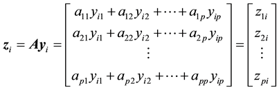
PCA is generally used for one sample without grouping among the observations, and the technique seeks to find the maximum of the variance of a linear combination of the variables [37] - [41] . The maximum of the variance of a linear combination of the variables is the first principal component, and the second principal component is perpendicular to the first principal component with the maximal variance of the linear combination of the variables. This process keeps going until it finds p principal components, where p is the number of variables [40] .
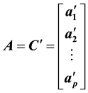
The principal components of the transformed variables are shown with the normalized eigenvectors  of the sample covariance matrix S of the sample of observation vectors
  [40] :
 (1)
(1)
where  is the jth normalized eigenvector of S and C is the orthogonal matrix consisting of
 ,
,
 (2)
(2)
According to Rencher and Christensen [40] , the eigenvalues  are obtained from S, and
  is the biggest eigenvalue of S. The first principal component
  shows the largest sample variance, whereas the variance of the last principal component
  is the smallest. Since the eigenvalues are equal to the variances of the principal components, the percentage of variance explained by the first
  principal components is as follows:
 (3)
(3)
We only expect to substitute the variables  for the first principal component

which accounts for more than 80 percent of the total variance4 since the dependent variables of air pollutants emissions are highly correlated with each other [42] - [44] . If this case is established, then a concept of a line segment is introduced to develop an AAQI in the transportation sector: 1) list all measurements calculated from the first principal component on a line segment and then find the maximum and minimum measurements, which are the most polluted and the least polluted observations, respectively; 2) measure the length of the line segment between the maximum and minimum measurements; and 3) calculate a proportion for each measurement from the ratio of the length of the line segment between the minimum measurement and each measurement to the length measured in 2), and then multiply the calculated values by 100. The least polluted observation indicates 0, while the most polluted observation indicates 100.
In Figure 1, this study illustrates a simple example to calculate an AAQI. Four measurements Z11, Z12, Z13 and Z14 are calculated from the first principal component representing the levels of multiple air pollutants. The
length of the line segment for each measurement is as follows: ;
; ; and
; and![]() . Therefore, the proportions of the four measurements are 0,
. Therefore, the proportions of the four measurements are 0, ![]() ,
, ![]() , and 1, respectively. The AAQIs for Z11, Z12, Z13 and Z14 finally are calculated as 0, 33.3, 66.6, and 100, respectively.
, and 1, respectively. The AAQIs for Z11, Z12, Z13 and Z14 finally are calculated as 0, 33.3, 66.6, and 100, respectively.
4. Data
An AAQI using PCA and the concept of a line segment was developed in Section 3 for multiple air pollutants. Under the Clean Air Act, the USEPA provides air quality standards for the five common air pollutants to suggest air quality guidelines to state policy planners and industrial sectors and protect public health [42] . For this reason, the five air pollutants of CO, NOx, PM, SO2, and VOCs were used for the index. Since principal components are not scale-invariant, all variables should be measured in the same units [3] ; therefore, all variables measured in tons were utilized by each transport mode in the 53 states in the US These were obtained from the NEI of the USEPA in 2008, and were the latest estimated air pollutants available during the study period [48] .
Table 1 shows the summary statistics for the data utilized in this study. The five air pollutants measured for each transport mode by state do not show any kind of heterogeneity since the coefficient of variation in each variable calculated was less than 10 [45] . For the airline transport mode, Texas emits the largest air pollution for each air pollutant, while District of Columbia shows the least air pollution. On the other hand, Idaho emits the fewest air pollutants for vessel and Louisiana shows the largest air pollution in CO, NOx, PM, and VOCs, but Texas is the largest SO2 emission state. For rail, Nebraska contributes to the largest air pollution across the nation for the four air pollutants, but Texas emits the largest SO2 emission as in the vessel case. For all five air pollutants, Rhode Island emits the least air pollution. For truck, California is the number one air pollution-emitting state for CO, NOx, and VOCs, while Texas is for PM and SO2. The least air pollution state for NOx, PM, and SO2 is Idaho, but that for CO and VOCs is Rhode Island.
Figure 2 provides a geographic map showing the study area where the five air pollutants were emitted. The NEI provides them by state, but there are no data available for some states for the vessel, rail, and truck transport sectors: Arizona, Colorado, Montana, North Dakota, New Mexico, Nevada, South Dakota, Utah, Virgin Islands, Vermont, and Wyoming in vessel; and Hawaii, Puerto Rico, and Virgin Islands in rail and truck.
5. Empirical Results
Like most multivariate analyses where the data used follow the multivariate normal (or at least approximately multivariate normal) distribution [46] , this study uses a multivariate analysis with PCA. Thus, the developed AAQI tests two statistical assumptions. The first assumption is of multivariate normality. In Figure 3, the scatter plot matrix on the left indicates that the original data do not suggest any normality and even each variable shows
![]() Z11(−5) Z12(−1) 0 Z13(+3) Z14(+7)
Z11(−5) Z12(−1) 0 Z13(+3) Z14(+7)
Figure 1. Line segment to calculate an AAQI of the example.
![]()
Table 1. Summary statistics for the five air pollutants emitted by the four transport modes.
Note: All air pollutants data come from the NEI in the USEPA [48] .
![]()
Figure 2. Geographic map showing the study area where the five air pollutants were emitted.
![]()
a positive skew. On the other hand, after the transformation of the original data5, the right side in Figure 3 shows the approximate normal distribution for each variable. The Q-Q plot for each variable does not show any distinct nonlinear relationship, not indicating a departure from the multivariate normality distribution [40] .
The second assumption is that this study can only use one principal component to sufficiently represent the five air pollutants![]() . To check this, the scree plots and proportion of variance explained by each principal component were tested (see Figure 4). The scree plots in all the transport modes reveal an evident natural break between the first and second principal components. Further, the proportion of the first principal component calculated6 shows more than 90 percent in each transport, which is much higher than a recommendation of retaining enough components to account for 80 percent of the total variance [40] . Being able to use only a first principal component to explain most of the total variance provides a significantly practical and convenient tool to interpret multiple air pollutants. For example, in the original data in 2008 by airline transport, two states, Iowa and Idaho, emitted the five air pollutants of CO, NOx, PM, SO2, and VOCs as follows: 2679, 272, 59, 37, and 119 (tons) and 3975, 255, 91, 35, and 147 (tons), respectively. In terms of individual air pollutants, Idaho emitted more (less) air pollution in CO, PM, and VOCs (NOx and SO2) than Iowa, but practitioners, state policy planners, and the public might want to know the overall air quality level from this kind of conservative situation. The first principal component calculated from the normalized eigenvectors of the sample covariance matrix was used to address this problem.
. To check this, the scree plots and proportion of variance explained by each principal component were tested (see Figure 4). The scree plots in all the transport modes reveal an evident natural break between the first and second principal components. Further, the proportion of the first principal component calculated6 shows more than 90 percent in each transport, which is much higher than a recommendation of retaining enough components to account for 80 percent of the total variance [40] . Being able to use only a first principal component to explain most of the total variance provides a significantly practical and convenient tool to interpret multiple air pollutants. For example, in the original data in 2008 by airline transport, two states, Iowa and Idaho, emitted the five air pollutants of CO, NOx, PM, SO2, and VOCs as follows: 2679, 272, 59, 37, and 119 (tons) and 3975, 255, 91, 35, and 147 (tons), respectively. In terms of individual air pollutants, Idaho emitted more (less) air pollution in CO, PM, and VOCs (NOx and SO2) than Iowa, but practitioners, state policy planners, and the public might want to know the overall air quality level from this kind of conservative situation. The first principal component calculated from the normalized eigenvectors of the sample covariance matrix was used to address this problem.
By using PCA and a little bit of algebra about a line segment with the transformed data, the first principal component and the AAQI by state in the airline, vessel, rail, and truck transport sectors were calculated, as shown in Table 2 and Table 3. In addition, to compare the relative levels of air quality by state from the indices, the state GDP in each transport mode was added in these tables. Each state is ranked relative to all other observed values of states in the first principal component, from smallest to largest in order of magnitude. The rank of each state is denoted by its AAQI. The index increases from 0 to 100, and this indicates more air pollution when it approaches a higher index value. The index of a state showing 100 means the largest air pollution-emitting state of all. On the other hand, a state index indicating 0 implies that the state is the least air pollution-emitting state.
![]()
Figure 3. Tests for departures from multivariate normality in the data set before and after the transformation.
![]()
Figure 4. The eigenvalues and proportion of variance explained by the first k principal components by each transport mode (k = 1, 2, 3, 4, 5).
The AAQIs in Table 2 and Table 3 are on the ordinal scale; in other words, it is only possible to distinguish each state on the basis of the relative amounts of multiple air pollutants. For instance, in vessel transport in Table 2, the index of Iowa shows 34.01, while that of Kentucky is 70.55. This does not tell us whether the air pollution by vessel in Kentucky is twice more polluted than that in Iowa, but rather it is interpretable in the way that Kentucky shows worse air pollution in terms of considering multiple air pollutants than Iowa. In fact, in 2008 Iowa emitted 151, 786, 27, 46, and 17 (tons) of CO, NOx, PM, SO2, and VOCs, respectively, whereas Kentucky emitted a considerable amount of air pollutants: 1847, 11370, 441, 594, and 300 (tons).
In Table 2, the vessel and rail transport sectors are first analyzed. In vessel transport, Oklahoma is the least air pollution-emitting state, but Louisiana shows the largest air pollution. Indiana, Illinois, Missouri, North Carolina, West Virginia, and Tennessee account for a relatively low AAQI compared with their high GDP levels, whereas Alaska, Michigan, Wisconsin, and Washington hold high ranks in the AAQI compared with their low GDP levels. For rail transport, Delaware takes the lowest rank in the index and Nebraska accounts for the highest rank. Florida, Georgia, and Texas show relatively low air pollution against their high GDP level. Massachusetts, Maryland, Missouri, Oregon, and Pennsylvania in vessel transport, consisting of a similar GDP scale, are differently ranked in the AQI, and this happens to rail transport with Arizona, Colorado, Florida, Montana, Tennessee, and Washington.
In Table 3, as this study expected based on the original data for the airline transport sector, where Texas was the largest air pollution-emitting state with respect to the five air pollutants, the Texas AAQI now reaches the highest. By contrast, Delaware holds the lowest rank in the AAQI. Connecticut, Minnesota, and New Jersey emit relatively low air pollution compared with their high GDP levels, while Alabama, Alaska, Massachusetts, Mississippi, Tennessee, and Wisconsin hold high ranks in the AAQI against their relatively low GDP levels. In truck transport, Idaho is ranked the least air pollution-emitting state, which even shows a relatively high GDP level. Truck transport was a little conservative to choosing the largest air polluting state with multiple air pollutants in the original data between Texas and California, but California is chosen as the largest air pollution- emitting state and Texas is ranked right behind it. Florida, Georgia, Michigan, New Mexico, and North Carolina, showing relatively low GDP levels, hold a high rank in the AAQI, whereas Arkansas, Iowa, Nevada, Nebraska, North Dakota, and South Dakota are ranked low in the index compared with their high GDP levels. In airline,
![]()
Table 2. The first principal component and AAQI by state in the vessel and rail transport sectors.
Notes: Data on District of Columbia, Idaho, Kansas, Nebraska, and Puerto Rico by vessel and on Rhode Island by rail were not available after the data transformation; the state GDPs by vessel and rail were obtained from the United States Bureau of Economic Analysis, and measured in millions of dollars [47] ; the GDP of Alaska in rail transport shows 0, which is explained by the value being much lower than one million; * means a state showing a relatively low AAQI compared with its high GDP level; † indicates a state holding a high rank in the AAQI compared with its low GDP level; ° means that a state showing a GDP level similar to other states, but it is differently ranked to others in the AAQI.
![]()
Table 3. The first principal component and AAQI by state in the airline and truck transport sectors.
Note: Data on District of Columbia by airline transport were not available after the data transformation; * means a state showing a relatively low AAQI compared with its high GDP level; † indicates a state holding a high rank in the AAQI compared with its low GDP level; ° means that a state showing a GDP level similar to other states, but it is differently ranked to others in the AAQI.
Louisiana and Wisconsin, showing a similar GDP scale, are differently ranked in the AAQI, which also arises in rail transport with Missouri, New Jersey, North Carolina Washington, and Wisconsin.
6. Conclusions
Transportation is an essential part of the socioeconomic development of a nation, but it has been needed to accompany the undesirable output called air pollution even though advances in technology for modern transport have contributed to reducing air pollution emissions in comparison with past transport modes. On the other hand, the continuous increase in a clean air environment for public health and sustainable growth between current and future generations has had a positive effect on the transportation sector, corresponding to the growing tide of preserving and improving air quality over the past decades.
An easily understandable tool to measure the level of air pollution in the transportation sector by considering multiple air pollutants might raise awareness about clean air to the public, practitioners, state policy planners, and the government. In this study, an AAQI was developed to help prepare decision makers, which could rank a state according to different levels of multiple air pollutants. In the US empirical case, some states were shown as less polluted or more polluted in terms of the index, although their GDP levels for a transport mode were similar to each other. The authors would carefully guess that a possible hypothesis of these differences might be attributed to the degree of the use of eco-friendly transport, strictness of air quality standards, and differences in gasoline prices in their boundaries.
This study, however, has a limitation based on the use of the index developed. The index is only available for one sample, not multiple samples together, since each sample has its own different normalized eigenvectors of the sample covariance matrix according to PCA. Thus, the index value of the same state in different two samples by transport mode, e.g., in 2005 and 2008 if 2005 data were available cannot be theoretically compared with each other. However, one possible advantage of the AAQI developed here is that it can be applied to other numerous index development projects, not limited to the transportation sector.
Acknowledgements
This research was supported by Mountain-Plains Consortium, which is sponsored by the US Department of Transportation through its university Transportation Centers Program. The contents are sole responsibility of the authors. The authors would like to thank anonymous reviewers for their constructive comments.
Author Contributions
Jaesung Choi conceived of the research and wrote the paper. Ju Dong Park and Yong Shin Park analyzed the data and performed the multivariate analysis. All authors discussed and commented the results and implications.
NOTES
*Corresponding author.
![]()
1The Clean Air Act was enacted in 1963 and revised in 1970 and 1990 to establish national air quality standards in the US [37] .
2NEI is an estimate of air emissions from all air emissions sources from 2002 to 2011 every three years [42] .
3The updated calculation methodology for data in 2008 was not consistent with 2002 and 2005, and air pollution data in 2011 were not available during the study period.
![]()
4Deciding on the number of components followed a recommendation of retaining sufficient components to account for at least 80 percent of the total variance [40] .
5In an attempt to make the individual variables distributed more closely to a normal distribution and them distributed more closely to a multivariate normal distribution, the following variables were used in this study:![]() ;
;![]() ;
;![]() ;
;![]() ; and
; and![]() .
.
6The first principal component in airline: 93.4 percent; in vessel: 95 percent; in rail: 97.8 percent; and in truck: 97.3 percent.