A Comparison Study of Cavitating Flow in a Ventricular Assist Device Using Laminar and Turbulent Model ()
1. Introduction
Cavitation was first related to valves of a mechanical heart in the 1980s after a series of valve fractures of a particular valve were observed [1]. Since then, many experimental and computational efforts have been devoted to understanding the flow and its detrimental effects on long-term operations of ventricular assist devices or artificial hearts. It has been known that cavitation could result in damage of blood cells and, hence, increase the risk of thromboembolic complications found in patients implanted with a mechanical heart. Various techniques for in vivo and/or in vitro detection of cavitation have been developed in the past few decades [2-6]. From the physical point view, such cavitating phenomena arises partially due to the fact that the pressure surge and the water hammer effect happen in closing ventricular valve (see, e.g., [7]). The drastic transient pressure change resulted from the pressure surge makes the cavitation even worse and more complicated.
In addition to various physiological issues, many physical phenomena due to mechanical heart valve closure have also been studied experimentally. Wu et al. [8] developed a laser sweeping technique which was capable of monitoring the valve closing motion with microsecond precision. Their observations show that at valve closure, the water hammer pressure reduction in combination with the high energy squeeze jet formed an environment favoring micro cavitation inceptions. Lee et al. [9] studied cavitation dynamics for different mechanical mitral heart valves using a stroboscopic visualization technique. Their in vitro study revealed several sources of cavitation initiation, including occluder stop, inflow strut, and clearance. They also concluded that the effects of fluid squeezing and the streamline contraction are major factors inducing cavitation incipience. Biancucci et al. [10] used a mock circulatory loop and videotaped the valve motion and the fluid flow around it. They found that gas bubbles formed during valve operation in the low pressure region due to gaseous nuclei and the presence of CO2. More recently, the high density particle image velocimetry technique has been developed. Detailed flow description becomes possible. It was found that the rebound effect played a significant role in the cavitation formation [11]. Lim et al. [12] further employed the high-speed flow imaging technique to identify regions of cavitation and found that the temporal fluid acceleration played an important role on cavitation inception. All these findings provide important inferences in the design of mechanical heart valves.
With the advancement of computational fluid dynamics (CFD), the numerical simulation has become an important strategy in the industrial design process for verifying and validating new product designs. This is no exception in the design of mechanical heart valves and ventricular assist devices. Makhihani et al. [13] specified the valve closing motion which was measured in vitro as input data and used a CFD package to compute the flow field. They predicted the possibility of cavitation inception by observing whether the fluid pressures dropped below the blood saturated vapor pressure. Lai et al. [14] employed CFD model to analyze the valve closure process and successfully evaluated the effect of alternations in the valve tip geometry. They concluded that a decrease of the tip velocity in the last few degrees led to a significant reduction of the negative pressure magnitude and, hence, the possibility of cavitation. Later, Cheng et al. [15] extended the CFD study to three-dimensional cases and observed vertical flow development during the valve impact-rebound phase.
It is quite unfortunate that most computational studies were restricted to laminar flow simulations though it is well known that cavitation usually happens in a highspeed region where the flow is usually turbulent. Furthermore, the inception of cavitation is usually indirectly inferred by observing whether the pressure drops below the saturated vapor pressure. In fact, it is vital to develop turbulent flow computation strategies with more realistic cavitation models to cope more rigorously with the medical physical phenomenon. Recently, Huang and Chen [16] first proposed a k-w turbulent model and employed a more realistic cavitation model to analyze the cavitation inception and process during the valve closure. The computed cavitation time endurance agrees with that available in the literature. In the present study, we applied the similar strategy to simulate the flow of a mechanical heart valve closure and compared the results obtained by laminar and turbulent models.
2. Physical Problem
Shown in Figure 1, a two-dimensional bileaflet valve system in a channel is analyzed in the present study. The length and width of the channel is L and 2w, respectively. Point O is the pivot of the valve. The lengths from both valve ends to the pivot is  and
and , respectively. The gauge pressure variations at the inlet and outlet are specified as
  and
and , respectively. The angular position of valve is given by
 .
.

Figure 1. Physical domain of the problem.
Considering the cavitating effects, the two-dimensional governing equations can be expressed as
 (1)
(1)
and
 (2)
(2)
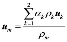
where  and
and  are the mixed density and velocity defined as
 (3)
(3)
( represents the volume fraction of phase k = 1 and 2 for liquid and gas phase, respectively) and
 (4)
(4)
respectively. Furthermore, p denotes the pressure and  the mixed viscosity
 (5)
(5)
The drift velocity
 (6)
(6)
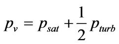
To find the fluid velocities and densities of liquid and gas phases, we employed the full cavitation model proposed by Singhal et al. [17]. This model employs a homogeneous flow approach and assumes that there are plenty nuclei for the cavitation inception. The following first-order effects are considered: the formation and transport of vapor bubbles, the turbulent fluctuations of pressure and velocity, and the magnitude of non-condensable gases. In the model, the phase-change vapor pressure is taken at
 (7)
(7)
where  is the saturation pressure of liquid and
  the turbulent pressure fluctuations
 (8)
(8)
with k being denoted the turbulent kinetic energy. The bubble growth and collapse is considered with the assumption of a zero velocity slip between fluid and bubbles. In addition, we also assume that the flow is isothermal and the fluid properties are constant in the whole flow domain. This implies that the cavitation is decoupled from heat transfer and radiation. For further elaboration of the bubble dynamics, please refer to [17].
Furthermore, to take account of the local turbulent flow effect, we used the k-w turbulence model which is more suitable to model turbulent flow at a smaller Reynolds number. The model employed in the present study is based on the results of Wilcox [18]. It is applicable to wall-bounded flows. For further elaboration of the equation systems taking cavitation into considerations, please refer to [16].
As shown in the governing equations, Equations (1) and (2), the mixture model is employed in the present study. The local velocity and density are functions of the volume fraction of vapor phase which is, in turn, controlled by the cavitation model through the bubble dynamics equation. Therefore, the local transition from laminar to turbulent flow can be influenced by the presence of cavitation. The interaction between the transition and cavitation is complicated and determined by the turbulence model, cavitation model, and the flow governing equations. Such an interaction could be an interesting fundamental issue but is beyond the present scope of study.
3. Numerical Method and Mesh Strategy
The commercial code FLUENT (version 6.3) was employed for the present study. In the code, the finite volume method was employed to discretize all differential equations and the algorithm of pressure implicit with splitting of operators (PISO) was adopted for nonlinear iterations of pressure and velocity solutions. The PISO algorithm is efficient and more accurate to solve the Navier-Stokes equations in unsteady problems because the momentum corrector step is performed more than once, compared to the traditional SIMPLE algorithm. The numerical procedures to compute the laminar and turbulent flows are identical except that the latter employed a turbulence model.
In the present study, the valve moves in time from a vertical position to a horizontal one. To cope with the motion, we employed a local dynamic mesh strategy which combines the spring-smoothing method and the local remeshing method. Shown in Figure 2, we divided the computational domain into three regions. In the regions away from and around the valve, a structured cartesian mesh was employed. The reason we used a structured grid around the valve is that it ensures better grid orthogonality and, hence, better solution quality in the region near the valve. In the region where the valve motion occurs, a non-structured mesh was generated.
With the valve motion, the mesh must be regenerated at each time step. However, since in computations, the time step is usually very small, it is not necessary to
remesh at every time step. Rather, we employed the spring-smoothing method to stretch and/or compress the local mesh near the valve in several consecutive time steps. When the local mesh becomes severely distorted, we remesh the grids around the valve. The grids near the valve at different times are shown in Figure 3.
4. Results and Discussions
In the following study, the geometric data we used for analysis are L = 38.1mm, w = 12.21 mm,  mm, and
  mm. The densities for liquid and gas are
  kg/m3 and
  kg/m3, respectively. Furthermore, their dynamic viscosities are
  kg/m×sec and
  kg/m×sec, respectively.
For comparison purposes, the specification of the inlet and outlet pressures and the valve rotation follows that in [14]. The inlet pressure  increases at a rate of 2 mmHg/ms from zero at t = 0 sec till it reaches 120 mmHg. The outlet pressure
  keeps at zero for all time. The valve is at its vertical position at t = 0 sec as shown in Figure 2 and rotates at a rate specified in [14].
After several tests, the appropriate time step is 
 sec. However, for a better resolution of cavitation phenomena, we require that
  sec.
sec.
4.1. Velocity Distribution before Cavitation
Figures 4 and 5 show the velocity distributions at different values of t for both the laminar and turbulent models, respectively. Due to the turbulence viscosity in the turbulent model, it is expected that the maximum velocity is significantly reduced in the turbulent flow simulation. Table 1 shows the maximum speed in the flow field at some particular time.
Figure 6 shows the maximum value variation of k with respect to time when we employed the turbulent flow model. Evidently, the flow is laminar at time t < 0.015 sec. Due to the increase of velocity, the flow begins to exhibit turbulent characteristic during 0.015 sec <