Application of Convolutional Neural Networks in Classification of GBM for Enhanced Prognosis ()
1. Introduction
Glioblastoma (also referred to as GBM) is a malignant brain tumor that is initiated as an addition and duplication of lethal cells (astrocytes) that lead to an eradication of healthy brain cells which can progressively worsen over time. It is mostly visible in the frontal and temporal lobes. GBM is classified as a grade IV astrocytoma (they are known to be very intrusive) [1] . It is one of over 120 types of various brain tumors that exist. Common symptoms a victim of Glioblastoma would experience include seizures, loss of memory, headaches, change in personality, nausea, etc. [2] . In a lot of cases, the cause of GBM is not known but in quite a few cases it is associated with genetics [2] . GBM is a fatal disease in most contingencies and there is no identified cure. However, the existing treatment/method of therapy is surgery and chemotherapy (radiation) [1] [2] . With the most neoteric advancements in the branch of machine learning artificial intelligence, Convolutional Neural Networks (CNNs) have become quite sought-after. CNNs convert images into arrays and matrices. It then utilizes various layers that act as filters which successively improve by executing high-quality detailing on images in the dataset. These networks operate on various arbitrary activation functions, the most favorable ones being the “Sigmoid” and “ReLu” activation functions. At its bare, cytoarchitecture identifies regional differences in the microstructural organization of the brain these neural networks work on the “Convolutional”, “Max Pooling”, “Flatten” and “Dense” layers that use extraction techniques to classify an image with a label (in most occurrences a 0 or 1). The method makes use of Python and a framework known as TensorFlow (Keras). This method can prove to be very effective in the field of medicine since neural networks have a successful classification rate of over 90%. STEM architecture could be revolutionary, and the research conducted can make a significant contribution to GBM research. The paper will be structured as follows: Literature Review, Data Collection, Experimentation, and then Conclusion.
2. Literature Review
2.1. Neural Networks
The researchers Macro, Claudio, and Enrico have researched Neural Networks and approaches to creating neural networks. It is primarily directed towards explaining the structure of neural networks (perceptrons, neurons, and layers). Their paper describes how Hornik’s theorem is applied to use a mathematical approach to acquire universal approximation properties. It also provides an in-depth analysis of arbitrary activation functions with relevance to output neurons. Various alternatives/approaches are listed. The first alternative consists of defining a quantum neural network as a variational quantum circuit composed of parameterized gates. Such quantum neural networks are empirically evaluated heuristic models of QML not grounded on mathematical theorems (more trial-and-error basis). However, the approach listed in the first alternative results in quantum algorithms suffering from an exponentially vanishing gradient problem (barren plateau problem). The second approach seeks to implement a truly quantum algorithm for neural network computations (using Hornik’s Theorem). The nonlinear activation function is again computed using the method of measurement operations [3] (Figure 1).
![]()
Figure 1. A representation of relation between one-layer perceptron and relative qubit-based version. Referenced from paper.
Each input neuron in the network corresponds to one qubit. The simplest way to achieve this is to simply store the data as a string of bits assigned to the classical base states of the quantum state space. The storage of a superposition of binary data as a sequence of bit strings in a multi-qubit state is a comparable 1-to-1 approach. Ultimately, the results derived from the experiment allow the implementation of a multilayered perceptron of arbitrary size in terms of neurons per layer as well as the number of layers [3] .
2.2. Convolutional Neural Networks for Cytoarchitectonic Brain Mapping
As regional variations in the arrangement and composition of neuronal cells are indicators of changes in connectivity and function, Christian, Hannah, Kai, Nina, Konrad, Alan, Stefan, Katrin, and Timo’s study examines the basic principles underlying the notion of cytoarchitecture and the microstructural organization of the brain. Automated scanning techniques are examined throughout the research, and observer-independent techniques are necessary to provide reproducible models of brain segregation and to accurately identify cytoarchitectonic zones [4] . Deep CNNs (Convolutional Neural Networks) are used to achieve this. The approach is founded on multivariate statistical image analysis, which has already been used to identify more than 200 regions. Properties are aggregated over numerous histological slices and different brains using cytoarchitectonic maps. The entire target brain area is divided into intervals of sections using the “divide & conquer” strategy, and these sections are surrounded with annotations that were made at roughly regular section intervals. Then, with the help of the enclosed annotations as training data, separate CNNs are trained for each interval. A group of local segmentation models are created as a result, each of which is tailored to automatically map just the tissue segments that fall inside the associated interval. Acquiring the datasets was the first step. The datasets used in this investigation include image collections of three human brains’ histological parts that have been stained for neuronal cell bodies [4] (Figure 2).
The cytoarchitecture, folding pattern, and staining characteristics of the brains differ. The following phase was developing local segmentation models. To train CNNs, also known as local segmentation models, cytoarchitectonic regions based on GLI mapping annotations were employed. Each local segmentation model was trained on two parts, which served as the training sections, and the target area’s accessible annotations. To “fill the gaps”, trained local segmentation models were then used. The model was then trained. Three thousand iterations of training were conducted. After 1000, 1400, 1800, 2200, and 2600 iterations, the learning rate was reduced by a factor of 0.5. The learning rate was initially set to 0.01 [4] . Depending on the network architecture (HR, LR, MS), the training environment (global vs. local segmentation models), the considered brain area, as well as the separation between annotated brain sections, differences in performance were seen. Except for LR (all), every architecture has comparably exceptional performance.
2.3. Classification Using DNNs for Brain Tumors
The study conducted by Heba, El-Sayed, and El-Harboty discusses how neural networks can be used to classify various brains into normal and different types
![]()
Figure 2. Division of mapped and unmapped intervals. Figure displays relationship between arbitrary functions, annotated intervals, and overall segregation. Referenced from paper.
of brain tumors. DNN classifier was used for classifying a dataset of 66 brain MRIs into 4 classes e.g. normal, glioblastoma, sarcoma, and metastatic bronchogenic carcinoma tumors. The classifier was combined with the discrete wavelet transform (DWT) the powerful feature extraction tool and the evaluation of the performance was quite good over all the performance measures. There is only one main approach listed. As opposed to shallow architectures like SVM and K-nearest neighbor (KNN), deep learning (DL) models may efficiently express complicated relationships without the need for a large number of nodes, setting an interesting trend in machine learning. [5] As a result, it will be applied to this specific study methodology in health informatics fields like bioinformatics, medical informatics, and medical image analysis. The proposed method trains the DNN classifier for the classification of brain cancers using a set of features retrieved using the discrete wavelet transform (DWT) feature extraction technique from segmented brain MRI images. The datasets are first acquired. The dataset is made up of 66 actual MRI scans of human brains, 22 of which are normal and 44 of which are malignant and represent metastatic glioblastoma, sarcoma, and bronchogenic carcinoma tumors, and was gathered from Harvard Medical School. Image segmentation is the subsequent stage. To distinguish between the many normal brain components, such as the gray matter (GM), white matter (WM), cerebrospinal fluid (CSF), and the skull in brain MR images, picture segmentation is a difficult task. Feature extraction and reduction are the following steps. Using the discrete wavelet transform (DWT), features of the segmented tumor are recovered after the Brain MR images have been divided into 5 pieces (Table 1).
The new methodology’s architecture is similar to that of convolutional neural networks (CNNs), but it uses less hardware and processes huge images in less amount of time. Comparing the classifier to more conventional classifiers, it exhibits great accuracy [5] .
3. Data Collection
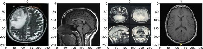
The data collected would have to be segregated into 2 different parts: MRI images of healthy brains and those of brains affected with Glioblastoma. The data will be scaled and pre-processed with correspondence to model requirements. The healthy dataset acquired has been found through the openBHB dataset. This
![]()
Table 1. Representation of the evaluation metrics for each type of machine learning algorithm. Useful in investigating the “best model” for training. Referenced from paper.
dataset is unique because the elements are extremely diverse (different ages, sexes, and settings). Additionally, the dataset is cleaned and preprocessed. The brain data for GBM brains have been compiled and are comprised of various scans conducted by clinics and world-renowned educational institutions. The data is then grouped into batches that have been assigned to labels (numerical binary values). In total, 131 brains correspond to the healthy brain category and 164 brains correspond to the glioblastoma category.
This data has then been split into 3 segments: the training set (accounts for 70%, batch length = 5), the validation set (accounts for 20%, batch length = 2), and the test set (accounts for 10%, batch length = 1). A scaled iterator is then created for the model to scan through batches, analyze the data using the trained model, and assign a label back.
4. Methodology
To conduct the experiment, TensorFlow, a popular open-source machine learning library, and Keras, its high-level API, were utilized. Data collection was then obtained and preprocessed according to model requirements. The batches are then assigned to labels [6] . A brain with GBM is classified with label “0” and a healthy brnain is classified with label “1”. The model was then constructed using a variety of layers, including convolutional (Conv2D), max-pooling (MaxPooling2D), dense (Dense), and flatten (Flatten) layers. The model was first assigned to the Sequential function. The neural network architecture was then constructed as follows: Image -> Conv2D -> MaxPooling2D -> Conv2D -> MaxPooling2D -> Conv2D -> MaxPooling2D -> Flatten -> Dense -> Dense.
As the input image passes through each layer of the model, the output shape and parameter count are modified. The initial output shape is (0, 254, 254, 16) with a parameter count of 448. Beyond this point, as the image is filtered, the shape tends to decrease while the parameter count increases (as progressively more batches are processed). GPU acceleration was also performed to reduce the amount of computer processing memory required [6] .
Now that the model is built with the various layers, it will then be trained on the processed and scaled data. The Depth, Height, and Width of the outputs have a great overall impact on the training ability (Figure 3).
![]()
Figure 3. Visual representation of the layers engineered in the Convolutional Neural Network. Shapes and type of layer are visually shown (along with input and output size of neurons).
A tensorboard will be created so that logs and informational numeric data will be stored in the array database (Figure 3). The model will be trained with 20 epochs and will be using the validation set at the same time. As the inputs are trained on each epoch, there is trend down in the loss and validation loss, and there is a trend upward in the accuracy and validation accuracy. The loss and accuracy plots are then plotted on a line graph as follows (Figure 4 and Figure 5).
The ReLu and Sigmoid function will also be applied in between the layers for enhanced scaled outputs. Metrics of the model performance are calculated with the following performance measures (in accordance to ŷ): Precision, Recall, and Accuracy. Once calculated, all of them returned a 1.0 (meaning 100%) which is an indicator of a successful experiment. An image at random is then given to the image based on a script, which returns a binary float between “0” and “1”. The benchmark set is 0.5 (meaning that the number will round and will be classified). To test the accuracy of the machine, an image at random (GBM) was given and returned an output of 0.4338, when rounded up it is assigned to label 0 (indicating that GBM is present).
5. Results
The approach involves the construction of a neural network using the machine learning libraries TensorFlow and Keras. The model architecture consists of multiple layers. These include the Conv2D, MaxPooling2D, Dense, and Flatten layers that are arranged sequentially [6] . As the input images proceeded to traverse through the model, noticeably, their shape and parameter count started to undergo changes. Initially, the output shape was observed to be (0, 254, 254, 16) with 448 parameters, subsequently also modifying in shape while the parameter count increased due to batch processing. The GPU acceleration effectively reduced the computational memory requirements during processing, this would have resulted in a longer training time. Throughout the training epochs, a quite consistent trend had emerged. It looked something similar to this: a decrease in both loss and validation loss, coupled with an increase in accuracy and validation accuracy. These trends were visually depicted through a plot representation
![]()
Figure 4. Loss plot using binary values when training over period of 20 epochs.
![]()
Figure 5. Accuracy plot using binary values when training over a period of 20 epochs.
(using matplotlib). Moreover, the useful integration of the ReLU and Sigmoid functions between layers really enhanced the model’s outputs. The 3 performance evaluation metrics—Precision, Recall, and Accuracy—were calculated based on the model’s predictions (ŷ). Through constant experimentation, it is observed that the model has consistently returned perfect scores of 1.0 (100%). In the process of assessing the model’s predictive ability, various random image inputs were utilized. When employing a standard benchmark threshold of 0.5 for the binary classification, the model had demonstrated an exceptionally high accuracy. For instance, a randomly provided image depicting GBM yielded an output of 0.4338, correctly classified as label “0”, signifying the overall presence of GBM. The constructed model had shown great performance in accurately discerning between the healthy brains and those afflicted with GBM. The accuracy metric on its own yielded a rounded figure of a whopping 96.98%. The consistently seen high precision, recall, and accuracy metrics validate the model’s overall effectiveness. This really supports the potential applicability of the model in clinical settings for identifying and distinguishing Glioblastoma.
6. Conclusion
Finally, the findings show that convolutional neural networks (CNNs) can be used to achieve 100% precision, recall, and accuracy in identifying cytoarchitectural differences in glioblastoma (GBM) images. This is a remarkable accomplishment because it suggests and establishes a path for CNNs to revolutionize the way GBM tumors are diagnosed and graded. Current diagnostic and grading methods for GBM tumors are invasive and time-consuming. They also necessitate a high level of pathologist expertise. CNNs could provide a more accurate and efficient method of diagnosing and grading these GBM tumors, potentially leading to better patient outcomes. It has the potential to be very useful in the most neoteric clinical trials.