High Sensitivity Digital Instantaneous Frequency Measurement Receiver for Precise Frequency Analysis

Bilal Abdulhamed^*, Chien-In Henry Chen

Department of Electrical Engineering, Wright State University, Dayton, Ohio, USA.

DOI: 10.4236/jcc.2024.121013                

Abstract

There are numerous applications, such as Radar, that leverage wideband technology. However, the presence of noise introduces certain limitations and challenges. It is crucial to harness wideband technology for applications demanding the rapid and precise transmission of diverse information from one point to another within a short timeframe. The ability to report a signal without tuning within the input bandwidth stands out as one of the advantages of employing a digital wideband receiver. As indicated, a digital wideband receiver plays a pivotal role in achieving high precision and accuracy. The primary distinction between Analog and Digital Instantaneous Frequency Measurement lies in the fact that analog Instantaneous Frequency Measurement (IFM) receivers have traditionally covered extensive input bandwidths, reporting one accurate frequency per short pulse. In the contemporary landscape, digital IFM systems utilize high-sampling-rate Analog-to-Digital Converters (ADC) along with Hilbert transforms to generate two output channels featuring a 90-degree phase shift. This paper explores the improvement of sensitivity in current digital IFM receivers. The optimization efforts target the Hilbert transform and autocorrelations architectures, aiming to refine the system’s ability to report fine frequencies within a noisy wide bandwidth environment, thereby elevating its overall sensitivity.

Keywords

Digital Wideband Receiver, Instantaneous Frequency Measurement (IFM) Receiver

1. Introduction

The Federal Communications Commission (FCC) defines any system with a transmission bandwidth exceeding 500 MHz as a wideband system. A notable advantage of wideband systems is their capability to transmit more data with lower power consumption [1] . In 2002, the FCC granted authorization for industrial companies to integrate wideband technology into commercial applications. One such commercial technology is Code Division Multiple Access (CDMA), which enables the utilization of a wideband channel by multiple narrowband channels [2] .

Wideband technology is widely employed in various commercial and electronic warfare applications. Wireless transmission of information from the transmitter to the receiver faces challenges from potential interruptions due to noise and distortion in the channel. While distortion is a fixed operation and can be straightforwardly addressed by applying the inverse operation, noise presents a more complex challenge due to its unpredictable nature. Different types of noise can partially or completely disturb the signal. Given that wideband technology operates with low power, noise becomes a significant issue for this technology. Consequently, this paper focuses on studying the enhancement of sensitivity and signal detection for a wideband receiver operating within a noisy wide bandwidth environment.

As the demand for increased data transmission in wireless systems continues to grow, wideband technology emerges as a promising candidate for the future of wireless communications. A defining characteristic of wideband systems is the occupied bandwidth, typically ranging from 500 MHz to 1 GHz. An important lesson from information theory highlights the significance of using appropriate coding to achieve a very low Binary Error Rate (BER) when transmitting data from one point to another [3] . This principle is effectively implemented when the data rate of the transmitted signal is lower than the capacity of the transmission line. Consequently, the capacity of a channel becomes a crucial indicator of the maximum achievable data rate within that channel. Wideband systems excel in monitoring multiple channels and detecting signals spread across them. Various types of receivers have been employed in general, contributing to the versatility of wideband technology [4] .

An analog IFM receiver depicted in Figure 1 cannot process multiple simultaneous signals where it processes only one signal; however, it has an accurate

Figure 1. Analog IFM receiver [6] .

frequency measurement, instantaneous bandwidth [5] . Because it requires a high signal to noise ratio in frequency measurement, the sensitivity of this receiver is low. Analog IFM receivers are often costlier and heavier than digital counterparts due to the complexity of analog components, complex manufacturing, customization needs, limited integration with digital technology, higher power consumption, and larger component size.

Digital systems provide unparalleled flexibility, enabling easy adjustments and optimizations through programmability. The integration of high-resolution components significantly enhances accuracy in frequency measurements. Leveraging sophisticated digital signal processing techniques adds a layer of noise immunity to the system, making it more resilient in challenging signal environments. Furthermore, the seamless communication enabled by integrating digital IFM with other digital systems enhances the overall efficiency of larger systems.

The advantages of the innovative approach presented in this paper revolve around the development of an IFM receiver that demonstrates exceptional performance even in highly noisy channels. The key strategy employed in this new approach involves leveraging Autocorrelation within the IFM receiver to mitigate the impact of noise on the signal. In essence, autocorrelation is utilized as a technique to analyze and identify patterns within the received signal, allowing the IFM receiver to distinguish the desired signal from the background noise. By incorporating autocorrelation into the design, the new digital IFM receivers exhibit notable benefits, particularly in scenarios where adaptability, advanced signal processing, and reliable performance in the presence of noise are crucial requirements even when confronted with significant levels of noise interference. Overall, the incorporation of autocorrelation in the IFM receiver enhances its resilience and effectiveness in challenging and noisy communication environments.

2. Proposed High Sensitivity Digital IFM Receiver

2.1. IFM Principle Operation

The core of the IFM receiver, the phase discriminator, takes in a radio frequency signal, divides it, and generates two separate signals. One signal is directed to the vertical plate, while the other is directed to the horizontal plate of a polar display. The estimation of the signal frequency is determined by calculating the angle.

The IFM Receiver operates on the principle of comparing two signals, one original and the other delayed by a phase discriminator (PD), to generate a precise output signal, aligning with IFM characteristics. The mathematical relationship between the phase difference of these signals is directly linked to frequency estimation.

The basic IFM receiver, depicted in Figure 2, comprises three essential components. The first part is a limiting amplifier designed to amplify low-power input signals and limit high-power signals. The second part is the frequency discriminator, which takes in received radio frequency signals, divides them, and generates two distinct signals. The frequency discriminator consists of three fundamental elements: the power splitter, delay line discriminator (DLD), and phase discriminator (PD). The accuracy of the DLD relies on the precision of the PD, ensuring accurate bandwidth and detected signal frequency. The third part of the IFM receiver is a polar display. If the output from the frequency discriminator (FD) applied directly into the horizontal and vertical plates of the polar display, the radial, and angular components can be calculated to read the received frequency immediately [7] .

2.2. IFM Design Considerations

The delay lines in the digital IFM receiver facilitate a phase comparison of the input signal for frequency calculation. The incoming signal is split into two signals, with one deliberately delayed by a specific time relative to the other. The basic delayed and undelayed block diagram is depicted in Figure 3.

There is always a phase difference between the outbound signal from the undelayed path and the delayed path, attributed to the constant time delay τ. In the digital IFM receiver, the frequency of the input signal can be calculated by determining the phase difference between the delayed and undelayed signals. If the phase angle (θ) is calculated, and the delayed time (τ) is known, the frequency of the input signal can be determined by:

$f=\frac{2\pi \tau }{\theta }$ (1)

Figure 2. Basic IFM receiver.

Figure 3. Signal paths of digital IFM receiver.

where, the phase angle (θ) can be calculated by:

$\theta ={\tan }^{-1}\left(\frac{E}{F}\right)$ (2)

where E and F are two voltages.

The radio frequency section of the IFM receiver consists of five main parts: a power divider, a delay line, a phase correlator (phase discriminator), four diode detectors, and two differential amplifiers. Figure 4 shows the block diagram of the radio frequency section of the digital IFM receiver.

The IFM receiver uses the power divider in order to divide the incoming received signal into two signals. The standard power divider part in the IFM receiver has one input and two outputs. The first output supplies the signal directly into the first input of the correlator. While the second output supplies the signal via the delay unit into the second input of the correlator. The correlator is used in order to perform the phase shifting on both the delayed and undelayed signals, and then combines them back. The four diodes or detectors are responsible about switching or converting the correlated input signals from standard RF signal into video signal. More than that, the four diodes or detectors are responsible for performing the mathematical multiplications signals by each other’s. The last component of the radio frequency section of the IFM receiver is responsible about performing the mathematical subtractions of the two signals.

The IFM receiver can estimate only one signal at a time. If the incoming signal to the IFM receiver is partially overlapped with another signal, the receiver will measure and estimate the strongest signal, potentially causing errors due to the influence of the other signal’s power. To address this issue and separate the power effect from the signal, a limiting amplifier is employed at the input of the IFM receiver. The use of a limiting amplifier enhances the sensitivity of the IFM receiver and renders the input power independent from the input signal [8] .

All components of the radio frequency section of the IFM receiver collaborate to execute the equations below:

$E=A\left(\omega \right)\sin \left(\omega \tau \right)$ (3)

$F=A\left(\omega \right)\cos \left(\omega \tau \right)$ (4)

Figure 4. RF section of the IFM receiver [8] .

These equations are employed in Equation (2) in order to calculate the phase angle (θ).

2.3. Proposed Digital IFM Signal Detection

The original digital IFM receiver operates by receiving the input signal and dividing it into two parts, namely real and imaginary components. This division is achieved through signal shifting or delay for a specific number of bits, a process carried out within the Hilbert transformer block. The output from the Hilbert transformer is directed to the autocorrelation block, generating five distinct delayed lines (S1, S2, S8, S32, S128) for each real and imaginary part. The results from the autocorrelation block are then input into the phase mapping block, which combines the delayed values to produce five phase delays or angles (Phase01, Phase02, Phase08, Phase32, Phase128). The output of the phase mapping block is subsequently fed into the frequency detection block, where the signal frequency is calculated using the equation below [9] :

$\text{SignalFrequency}=\frac{\text{Freuency}128}{2\pi }\times 2.56\times {10}^9$ (5)

Signal frequency is estimated through an indirect mathematical calculation.

The IFM detection variable is determined using the output values of the autocorrelation algorithm, and it can be calculated using the formula below [9] :

$\text{DetectionVariable}={\displaystyle {\sum }_{m}S{\left(m\Delta t\right)}^{\prime }\times S\left(m\Delta t\right)}={\displaystyle {\sum }_m{C}_m^2}$ (6)

where the m represents the delay numbers (1, 2, 8, 32, 128) while t represents the time.

The essential of the entire process lies in dividing the received signal into two parts and then combining them to obtain the phase or angle of that frequency. The initial step, following the extraction of the complex signal from the Hilbert transform, involves calculating the first phase shift. Two parts are processed to derive the first phase shift: the first part results from shifting the complex signal by one bit to the right, and the second part results from shifting the complex signal by one bit to the left. Subsequently, the two parts are summed and convoluted to generate the first signal, S01. The phase or angle can be computed using the formula provided below [9] :

$\text{DetectionVariable}={\tan }^{-1}\left(\frac{\text{Imaginary}\left(Q\right)}{\text{Real}\left(I\right)}\right)$ (7)

Equation (7) is employed to calculate the phases of the signals. Figure 5 shows how the process of calculating the first phase shift is done:

where length: m = 1, and Delay = 256.

The computed phase or angle is utilized to calculate the first frequency using the formula [9] :

$f_1=\frac{f_s\times Phase}{2m\pi }$ (8)

Figure 5. Process of calculating first Phase shift.

where f_s is sampling frequency = 2.56 × 10⁹.

The computed frequency is utilized to calculate the first Zone using the formula:

$Z_m=\text{floor}\left[\frac{m\times f_{m-1}}{f_s}\right]$ (9)

The computed Zone is utilized to calculate the second frequency where the frequencies “frequency 02, frequency 08, frequency 32, frequency 128” use the formula:

$f_m=\frac{f_s\times Phas{e}_m}{2\pi m}+\frac{2\pi f_s{Z}_m}{2\pi m}$ (10)

The equations Equation (9) and Equation (10) are utilized from m = 2 to the m = 128. The final result, denoted as frequency 128, is employed to calculate the more accurate frequency output, referred to as Signal Frequency.

Next, in the proposed new architecture, I adhere to the same procedure for calculating Phases, Frequencies, and Zones for m = 01, 02, 08, 32, 128. The primary distinction between the original and the new architecture lies in the Hilbert Transform, as well as the shifting and delaying of the output from the Hilbert transform.

3. Proposed IFM Architecture

The fundamental structure of the digital IFM receiver will remain consistent. However, specific modifications and alterations will be introduced to the internal design and architecture of the Hilbert Transform component.

The overall framework of the digital IFM receiver, as depicted in Figure 6, will serve as the foundational structure, ensuring continuity in its operational principles and functionalities.

The internal architecture of the Hilbert transform (HT) is depicted in Figure 7.

The internal architecture of the autocorrelation algorithm, phase mapping, and frequency detections that are employed in the digital IFM receiver are depicted in Figure 8.

The original autocorrelation process involves a delaying and shifting procedure based on the deletion of bits, followed by autocorrelating the result. To illustrate this process, let’s consider a scenario with a total of n = 256 bits and

Figure 6. Digital IFM architecture [9] .

Figure 7. Hilbert transform [9] .

Figure 8. Autocorrelation algorithm.

sample delays m = 2 and m = 128. In this case, the first part of the complex signal is generated by removing the last two bits of the stream (bits 255 and 256). Conversely, the second part is created by deleting the first two bits of the stream (bits 01 and 02).

This results in a stream of 254 bits. When the number of sample delays is m = 128, the process produces a stream of 128 bits. Essentially, the autocorrelator doesn’t correlate all received data; instead, some bits are deleted based on the number of sample delays. Figure 9 provides a detailed representation of the shifting and deleting bits process performed by the original Hilbert,

Figure 9. Original Hilbert delay line.

preparing a stream for autocorrelation.

The new Hilbert transform delay adopts a strategy of shifting the entire stream rather than deleting data. To illustrate this process, let’s consider a scenario with a total of n = 256 bits and sample delays m = 2 and m = 128. In this case, the first part of the complex signal is generated by shifting the entire stream two bits to the right (from bit number 3 to bit number 258), resulting in a stream of 256 bits. Similarly, when the number of sample delays is m = 128, the same process is applied, producing another stream of 256 bits. In contrast to the original Hilbert, the new Hilbert process involves processing all received data without deleting any bits. Figure 10 outlines the process of shifting bits performed by the new Hilbert, preparing a stream for autocorrelation.

The new Hilbert Transform incorporates crucial and precise processing steps on the received signal to enhance the detected data and achieve the most accurate signal representation. Initially, the incoming data is divided into two separate lines. The first line is responsible for generating the real part and undergoes a process of shifting the received data six bits to the left using Z transform. Meanwhile, the second line initiates its process by dividing the data into an 11-bit queue through the application of an 11-Tap Finite Impulse Response (FIR) filter. The FIR filter execution involves multiplying the 11-bit data by corresponding coefficient values [6 0 10 0 30 0 −30 0 −10 0 −6].

The example provided demonstrates the functioning of the 11-Tap FIR, where the inputted data [1 1 0 1 1 0 0 1 0 0 1 1 0 0 0 1] undergoes the entire process, yielding the final result.

In Figure 11, the entire input data undergoes a one-place shift for each cycle. The results are determined by multiplying the FIR coefficients with the values present in each row. The equation below illustrates how the results are calculated:

Figure 10. New Hilbert delay.

Figure 11. Input and output of 11-Tap FIR.

$\begin{array}{l}6\times \text{firstbit}+10\times \text{Thirdbit}+30\times \text{fifthbit}-30\times \text{seventhbit}\\ -10\times \text{ninthbit}-6\times \text{eleventhbit}\end{array}$ (11)

Since the coefficient of the 11-Tap FIR has five zeros, the first five bits of the results will be ignored. The primary function of the digitizer block is converting negative values into 1 and the zeros or positive values into 0. To meet the requirements of the 11-Tap FIR, every 512 cycles are shifted to left by five bits. The shifted five bits represent the number of zeros that are used in the 11-Tap FIR filter coefficient. As the output of the digitizer is one-bit data, it is then converted into 512-bit data by using the parallel-to-serial converter. Figure 12 shows how the digitizer works:

The next step involves autocorrelation where the real and imaginary parts are correlated. The original autocorrelation process relies on correlating the complex value shifted to the left by a specific number of bits with the complex value shifted to the right by the same number of bits. For instance, the autocorrelation of the second signal is illustrated below:

where n = 256, pp = m = 2.

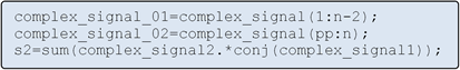
In the new Autocorrelation process, the correlation involves correlating the shifted complex value to the left by a certain number of bits with the original complex signal. For instance, the autocorrelation of the second signal is as follows:

The main difference between the original and the new autocorrelation process is that the original architecture is built on correlating two shifted complex signals, while the new architecture is built on correlating the shifted signal with the original complex signal. Figure 13 and Figure 14 show the original and new autocorrelation processes:

4. Threshold Determination and Precise Frequency Analysis

The original architecture of the digital IFM receiver generates a relatively low

Figure 12. Digitizer.

Figure 13. Original autocorrelation.

Figure 14. New autocorrelation.

Figure 15. Results of original IFM when SNR = −3 dB.

threshold, which often lacks accuracy. The received signal is acceptable for SNR = 0, SNR = −1, and SNR = −2. Occasionally, the detected signal might be acceptable for SNR = −3, but this is contingent on the random noise introduced into the signal. Figure 15 illustrates the outcomes of the original IFM architecture when SNR = −3 dB.

Left side plots of Figure 16 illustrates the correlation between the normalized frequency of the signal and the input frequency, while right side plots of Figure 16 depicts the relationship between the offset frequency of the signal and the input frequency [10] . The new architecture of the digital IFM receiver has significantly enhanced the overall response, nearly doubling its effectiveness. The response of the new architecture extends to SNR = −7 dB, surpassing the performance of SNR = −3 dB. In certain instances, the improvement even extends to SNR = −8 dB, contingent on the presence of random noise. Figure 16 showcases the response of the new architecture at SNR = −3 dB and SNR = −7 dB.

Figure 16. Results of new IFM when SNR = −3 & −7 dB.

5. Conclusions

The modification to the internal mechanism of the Hilbert Transformer has yielded significant improvements in both the sensitivity and performance of IFM system. Notably, these enhancements empower the IFM to operate effectively in environments characterized by dense and robust noise. To validate these improvements, comparative testing was conducted, subjecting both the original Hilbert transformer and the enhanced version to the same parameters and circumstances.

In a test scenario with an exceptionally high instantaneous frequency bandwidth of 1.2 GHz, the new mechanism of the IFM demonstrated its efficacy, showcasing its adaptability for wideband receiver applications. The comparison between the original and modified mechanisms revealed compelling results. When employing the original IFM mechanism, the frequency offset between the estimated and original frequencies was 300 MHz at a Signal-to-Noise Ratio (SNR) of −3 dB. In contrast, the proposed IFM mechanism achieved a remarkable reduction in frequency offset, with values within 2 MHz at an SNR of −7 dB.

This improvement in sensitivity can be attributed to a key enhancement: the utilization of all received data in the autocorrelation process for frequency estimation. The IFM’s response and sensitivity have undergone a notable enhancement, resulting in an improvement of nearly 4 dB. These advancements signify a substantial leap forward in the IFM receiver’s ability to accurately estimate frequencies, especially in challenging and noisy environments.

Future work includes leveraging autocorrelation and cross-correlation techniques to identify and extract signal patterns in the presence of noise. These techniques help in enhancing the signal-to-noise ratio and improving overall sensitivity. Subsequently, the integration of machine learning becomes imperative—implementing machine learning algorithms to learn and adapt to the characteristics of received signals and noise patterns. Machine learning models have the potential to augment the receiver’s ability to recognize and effectively filter out noise. Lastly, there is a focus on implementing dynamic thresholding mechanisms capable of adapting to changing noise levels. This adaptive approach ensures that the receiver maintains optimal sensitivity under varying environmental conditions.

Conflicts of Interest

The authors declare no conflicts of interest regarding the publication of this paper.

References

[1]	Tsui, J.B.-Y. (2001) Digital Techniques for Wideband Receivers. 2nd Edition, Artech House Radar Library, Boston.
[2]	Wilson, L.A. (1987) BRAGG-CELL Receiver Study. Jet Propulsion Laboratory, California. https://apps.dtic.mil/sti/pdfs/ADA189361.pdf
[3]	Cheng, C.-H., Lin, D.M. and Tsui, J.B. (2012) Electronic Warfare Receiver with Multiple FFT Frame Sizes. IEEE Transactions on Aerospace and Electronic Systems, 48, 3318-3330. https://doi.org/10.1109/TAES.2012.6324709 https://www.researchgate.net/publication/260514129_Electronic_Warfare_Receiver_with_Multiple_FFT_Frame_Sizes
[4]	Myburgh, K. (2015) The Design and Development of a Co-Pulse IFM Receiver. Master’s Thesis, Stellenbosch University, Stellenbosch. https://scholar.sun.ac.za/server/api/core/bitstreams/93b122c6-82aa-4d6d-9316-e2499ae7db33/content
[5]	Tsui, J.B.-Y. (2005) Microwave Receivers with Electronic Warfare Applications. A Wiley-Interscience Publications, North Carolina.
[6]	Norouzi, Y., et al. (2017) Performance Analysis of Mono-Bit Digital Instantaneous Frequency Measurement (Difm) Device. https://api.semanticscholar.org/CorpusID:55235832
[7]	Johansson, M. (1999) The Hilbert Transform. M.Sc. Thesis, Växjö University, Växjö.
[8]	Pandolfi, C., et al. (2010) Comparison of Analog IFM and Digital Frequency Measurement Receivers for Electronic Warfare. The 7th European Radar Conference, 232-235. https://api.semanticscholar.org/CorpusID:36133423
[9]	Helton, J., Chen, C.H., Lin, D.M. and Tsui, J.B. (2008) FPGA-Based 1.2 GHz Bandwidth Digital Instantaneous Frequency Measurement Receiver. 9th International Symposium on Quality Electronic Design (ISQED 2008), San Jose, CA, 17-19 March 2008, 568-571. https://doi.org/10.1109/ISQED.2008.4479798
[10]	Elisra Electronic Systems Ltd., Microwave Division Bene Beraq, Israel (2007) A Digital Instantaneous Frequency Measurement Receiver. Microwave Journal. https://www.microwavejournal.com/articles/4772-a-digital-instantaneous-frequency-measurement-receiver