Financial Anomalies and Creditworthiness: A Python-Driven Machine Learning Approach Using Mahalanobis Distance for ISE-Listed Companies in the Production and Manufacturing Sector

Hasan Demirhan

The Graduate School of Social Sciences (GSoSS), Ankara University, Ankara, Türkiye.

DOI: 10.4236/jfrm.2024.131001                

Abstract

This paper investigated the effect of financial ratio anomalies on the creditworthiness of companies in the production and manufacturing sectors listed on the Istanbul Stock Exchange. Financial ratios are crucial in assessing creditworthiness as they reflect potential financial risks, but anomalies in these ratios can skew credit evaluations. The statistical analysis is carried out using the Mahalanobis distance, a Python-driven machine learning technique, with financial data from 254 companies over the period of 2014 to 2023. The findings show that 89.61% of the observations were identified as normal, falling into low and moderate risk categories, whereas 10.39% were considered anomalies or high-risk, indicating that a substantial proportion of companies maintained financial indices within expected ranges. Besides the study observed significant risk category variations, particularly in the latter half of each year, likely reflecting differing reporting and auditing practices. Farther, Principal Component (PCA) analysis indicated that Asset Profitability, EBITDA to Total Debts, Short-Term Debt to Current Assets, Net Sales to Short-Term Debts, and Current Ratio are the most influential financial ratios. On the other hand, the least influential financial ratios in PCA include Net Working Capital Turnover, Operating Expenses to Average Assets, Market Value to EBITDA, Efficiency Ratio (Assets Turnover Ratio), and Change in Depreciation Expenses Ratio (annual difference in depreciation expense). In conclusion, this study underscores the complex role of financial ratio anomalies in Turkish industries in assessing creditworthiness.

Keywords

Financial Ratios, Mahalanobis Distance, Principal Component Analysis, Anomaly Detection, Financial Risk Categorization, Creditworthiness

1. Introduction

In recent years, the global financial landscape, including the Turkish economy, has been marked by volatility, accentuated by events such as the COVID-19 pandemic. The Istanbul Stock Exchange (ISE), now known as Borsa Istanbul, is a central player in this landscape, particularly for companies in the production and manufacturing sectors. These companies have navigated challenges arising from local operational difficulties and fluctuating global demand. The ISE, as Türkiye’s primary financial marketplace, is not only a barometer of the country’s economic health but also a crucial platform for both domestic and international investors. This study focuses on the production and manufacturing industries, providing insights into corporate resilience and financial solidity.

Creditworthiness, defined as a company’s ability to meet its financial obligations, is a fundamental metric for stakeholders like lenders and bondholders. It indicates the likelihood of default and is pivotal in determining a company’s access to capital and borrowing costs. This is particularly vital for capital-intensive sectors like production and manufacturing. Consequently, understanding and evaluating creditworthiness is essential, not only to maintain investor confidence but also to reflect a company’s financial health. Within this context, even minor irregularities in financial indicators can signal broader economic trends or potential financial mismanagement.

Financial ratios, serving as key indicators of a company’s performance and health, are essential for informed decision-making by investors and analysts. Anomalies in these ratios, therefore, warrant close examination as they can reveal underlying issues affecting a company’s financial status. This study adopts a sector-specific approach, concentrating on the production and manufacturing sectors of the ISE. Such a focus allows for a more nuanced understanding of the financial health and performance metrics pertinent to these sectors, yielding benefits like enhanced comparability, data homogeneity, and sector-specific insights.

The aim of this study is to investigate the relationship between financial ratio anomalies and credit quality among ISE-listed companies in the production and manufacturing sectors. Utilizing financial data from Q4 2014 to Q1 2023 of 254 companies, the research employs Python-based machine learning techniques to uncover insights beyond the scope of traditional analysis. The study encompasses the examination of various financial ratios, identification of anomalies, and assessment of their impact on credit quality, thereby providing valuable insights for stakeholders in these sectors.

At the heart of this methodological innovation is the use of the Mahalanobis distance, a multivariate statistical tool, to identify patterns of anomalies in financial ratios. These patterns may indicate managerial inefficiencies, fraudulent activities, or reporting inaccuracies. By analyzing these outliers against sector-specific trends and economic conditions, the study adds a predictive dimension to credit risk assessment.

Moreover, the paper extends the concept of “distance” to quantify the severity of an anomaly, thereby facilitating a ranking of each company’s creditworthiness based on their financials. The integration of dimensionality reduction techniques like Principal Component Analysis (PCA) with the Mahalanobis distance not only refines the anomaly detection model but also provides deeper insights into the financial data. Therefore, the combination of PCA and Mahalanobis distance, as explored in this study, represents an innovative approach to detecting financial anomalies and evaluating creditworthiness, promising to add a new dimension to the field of financial analytics.

It is essential to clarify that this paper employs the term “anomaly” rather than “fraud” (Hawkins, 1980) . “Anomaly” refers to deviations from normative data patterns, which may not always stem from deliberate deceit. Due to the scarcity of reliable data on fraudulent activities, particularly in the Turkish market, and the legal implications of labeling such irregularities as “fraud”, this study focuses on “anomalies”. Nonetheless, identifying these anomalies can lead to further investigations that might uncover fraudulent activities or financial vulnerabilities, building upon analytical techniques from fraud detection literature (Agrawal & Cooper, 2017) . Thus, while the term “anomaly” is employed for its broader definition, the methodologies are informed by advanced fraud detection approaches.

2. Literature Review

This literature review delves into the multifaceted areas of financial ratio anomalies, the emergent role of machine learning in finance, and the application of the Mahalanobis distance within creditworthiness assessment. It acknowledges the expanding field of financial analytics that increasingly adopts sophisticated machine learning techniques to decipher complex financial data patterns. This review particularly focuses on the integration of feature importance analysis, dimensionality reduction techniques such as Principal Component Analysis (PCA), and the utilization of Mahalanobis distance in the nuanced task of detecting financial anomalies and assessing creditworthiness (Lokanan et al., 2019) .

Principal Component Analysis (PCA) has been a cornerstone in finance for reducing the complexity of financial datasets while retaining essential information. Jia et al. (2022) have demonstrated the effectiveness of PCA in distilling complex financial datasets, thus enhancing the computational efficiency of subsequent analyses. Complementing this, Davis & Pesch (2013) have illustrated how PCA can unearth hidden factors in financial data, which are typically obscured in high-dimensional spaces.

The topic of financial ratio anomalies has captivated researchers for several decades. These anomalies represent inconsistent or unexpected patterns in financial ratios that defy explanation by traditional financial theories. Pioneering studies have sought to understand the roots and ramifications of these anomalies, with factors like data inconsistencies, corporate financial policies, and market inefficiencies frequently cited. Seminal works in this domain have investigated anomalies in relation to predicting stock returns, corporate bankruptcy, and the impacts of seasonal variations in financial reporting. The identification and interpretation of these anomalies are imperative for investors and analysts striving to make informed decisions.

Financial ratio analysis is a fundamental aspect of financial assessment for companies, providing insights into their performance, stability, and creditworthiness. Seminal contributions by Beaver (1968) regarding financial ratios and the prediction of corporate bankruptcy laid the foundation for further research into financial anomalies. This trajectory was significantly advanced by studies such as Altman (1968) ’s introduction of the Z-score model, which has been seminal in elucidating the predictive power of financial ratios for corporate failures. The primary emphasis in the literature has been on the development of models for predicting bankruptcy. These models are tailored to a wide array of sectors, including manufacturing, banking, airlines, small businesses, and the oil and gas industry. To forecast bankruptcy across these varied markets, financial ratios are commonly employed within multi-discriminant analysis and logit models, demonstrating a notable degree of accuracy (Giannopoulos & Sigbjørnsen, 2019) .

In the realm of financial ratio analysis and anomalies, feature selection emerges as a critical factor in financial modeling. It significantly influences both the interpretability and accuracy of predictive models. Wasserbacher & Spindler (2022) have highlighted the necessity of pinpointing salient features in financial datasets to boost model efficiency and predictive accuracy. Furthering this perspective, Jones (2023) has elaborated on how feature importance analysis can substantially reduce noise and enhance the relevance of data inputs in financial forecasting models.

Regarding Türkiye, the study by Tarim & Karan (2001) , which examined the relevance of financial ratios in predicting company performance in Turkish industries, is particularly noteworthy. Additionally, research like that of Ertuğrul & Karakaşoğlu (2009) has investigated the predictability of financial ratios for firm performance on the ISE. However, specific research addressing anomalies in these ratios is scant but nonetheless provides a crucial reference for understanding historical applications within the Turkish context.

The integration of machine learning (ML) techniques into financial analysis represents a pivotal advancement. Recent surveys, such as the one by Barboza et al. (2017) incorporate ML applications for credit risk analysis, showcasing the breadth of ML’s impact. The adaptability of machine learning algorithms in interpreting intricate patterns in financial markets has been accentuated by studies like those of Wang et al. (2018) . They further highlight how Python-driven machine learning approaches have introduced more nuanced and sophisticated analytical capabilities into financial analysis.

Sector-specific research also deserves acknowledgment. For instance, Kumar & Ravi (2016) have conducted notable work on financial performance prediction in the manufacturing sector using machine learning. In a different vein, the study by Siami-Namini et al. (2018) forecasts agricultural economics and risks, offering insights into the application of ML in this sector.

The evolution of computational technology has elevated machine learning (ML) to a crucial tool in financial analysis. Fintech has widely adopted ML for diverse tasks, from credit scoring to market prediction. Previous studies like that of Liu et al. (2021) have successfully applied ML techniques to financial ratio analysis for credit risk evaluation. Within the production and manufacturing sectors, the applicability and efficacy of ML in interpreting financial ratios for creditworthiness have been highlighted by Trivedi (2020) and Tripathi et al. (2021) . However, this area remains a growing field in Turkish-specific research.

2.1. The Mahalanobis Distance

The Mahalanobis distance, first introduced by Mahalanobis in 1936, is a statistical measure recognized for its efficacy in identifying multivariate anomalies. While its application in finance is a relatively recent development, it has garnered increasing attention for its potential in outlier detection within financial datasets. Markopoulos et al. (2015) have underscored its utility in this context, particularly noting its unexplored potential in analyzing financial ratios of manufacturing and agricultural companies.

The use of Mahalanobis distance in finance, though less common, has been explored in various studies. An early example of its potential is found in the work of Deakin (1972) , who applied it to detect corporate financial fraud. Lokanan et al. (2019) further revealed its value, highlighting its sensitivity to covariance among variables, making it particularly adept at detecting subtle anomalies in financial datasets. These anomalies, in financial contexts, could be indicative of significant events like fraud or market crashes.

Earlier studies, even if not explicitly employing the Mahalanobis distance, have utilized similar statistical techniques in financial analysis and creditworthiness assessment. For instance, methods like cluster analysis, principal component analysis (PCA), and discriminant analysis, which adhere to the Mahalanobis principle of considering the variance-covariance structure of data, have seen widespread application in finance.

The integration of PCA with Mahalanobis distance for anomaly detection in finance, though not extensively explored in existing literature, presents an area ripe for research. Wang et al. (2020) provides a conceptual framework discussing this integration’s potential in enhancing anomaly detection systems’ accuracy. They suggest that the conjunction of PCA’s data condensation capabilities with the Mahalanobis distance’s sensitivity to multivariate relationships could yield a more effective anomaly detection mechanism in financial datasets.

2.2. Turkish-Specific Financial Studies

This section of the literature review addresses the integration of financial ratio anomalies, machine learning in finance, and the application of the Mahalanobis distance within the specific context of the Turkish production and manufacturing sectors. There is a notable gap in the comprehensive research that combines these elements for companies listed on the Istanbul Stock Exchange (ISE). This gap presents an opportunity for innovative research utilizing a Python-driven ML approach, leveraging the Mahalanobis distance to contribute significantly to financial literature and creditworthiness assessment mechanisms for ISE-listed companies.

In Turkish financial research, advanced statistical methods that resonate with the principles of the Mahalanobis distance have been implemented. Researchers have employed various multivariate techniques that analyze correlations among multiple financial indicators to gain insights into firm performance and credit risk. While these studies might not explicitly mention the Mahalanobis distance, they often use related concepts like multivariate outlier detection or covariance-based classification. For instance, Ertuğrul & Karakaşoğlu (2009) used the TOPSIS method in their study on Turkish cement firms, a technique akin to the Mahalanobis distance in its consideration of the variances and covariances of different criteria. Moreover, Öğüt et al. (2012) in their work on predicting bank financial strength ratings employed a methodology that mirrors aspects of the Mahalanobis distance, particularly in how multiple correlated financial variables are used to predict financial strength and stability.

Regarding empirical applications, the research by Demir & Gök (2018) , on bankruptcy prediction using machine learning algorithms is particularly relevant. Although primarily focused on machine learning, their work aligns with the concept of anomaly detection, which is central to the Mahalanobis distance. These models, by identifying patterns that deviate from expected norms, encapsulate the core idea of detecting anomalies based on historical financial data.

In concise, while the Mahalanobis distance is not frequently cited directly in Turkish financial analysis, the statistical principles it embodies are evident in various methodologies employed to dissect financial data intricacies. The versatility of these statistical techniques in detecting financial anomalies and assessing creditworthiness provides a solid foundation for further exploration and justification of the Mahalanobis distance’s application in the Turkish financial context.

3. Overview of the Industrial and Manufacturing Sectors in Türkiye

Türkiye’s industrial sector has been integral to its economic growth and development, particularly over the last few decades. The country embarked on an ambitious journey of industrialization in the mid-20th century, initially propelled by a state-driven, import-substitution model (Berument & Taşçı, 2002) . The foundation for industrial expansion was set with the establishment of the State Economic Enterprises (SEEs) in the 1950s. A significant paradigm shift occurred post-1980 with the adoption of liberalization policies, pivoting towards an export-oriented strategy (Kepenek & Yentürk, 2005) . The 1995 Customs Union agreement with the EU further accelerated this process, embedding Turkish manufacturers into global supply chains (Öniş & Webb, 1992) .

The energy sector in Türkiye has undergone significant evolution in tandem with the country’s burgeoning energy needs, fueled by economic expansion. Initially dominated by coal and hydroelectric power, recent decades have seen a shift towards natural gas and renewable energy sources (Erdogdu, 2007) . The liberalization of the energy market in the 2000s, aiming to diminish state control, has not only drawn foreign investment but also enhanced sectoral efficiency (Mehmet & Yorucu, 2021) .

The Turkish consumer discretionary sector, encompassing automotive, retail, and durable goods industries, witnessed rapid expansion during the economic liberalization era of the 1980s. The post-2001 financial reforms, alongside globalization and domestic economic stabilization, catalyzed a surge in foreign direct investment, significantly bolstering this sector’s growth (Atiyas, 2013) .

In the realm of food production, Türkiye historically maintained self-sufficiency until the late 20th century. Urbanization and policy shifts promoting industrial agriculture have transformed the sector, leading to decreased employment in agriculture but heightened productivity (Kazgan, 2012) . Türkiye continues to be a key agricultural producer in the region, with a diverse export portfolio. The recent emphasis on sustainable practices and organic farming aligns with global consumer trends and the EU’s influence on agricultural standards.

In short, Türkiye’s production and manufacturing sectors have undergone profound transformations from their initial state-driven growth models to more liberalized and diversified frameworks. These transitions have been pivotal in shaping the country’s economic trajectory and its integration into the global economy.

3.1. Challenges of Turkish Production and Manufacturing Sectors

The industrial and materials sector in Türkiye has faced significant challenges, particularly in the wake of the COVID-19 crisis. Disruptions in international trade and production have exposed vulnerabilities in both global and local supply chains (Republic of Türkiye Ministry of Energy and Natural Resources, 2020) . Despite these obstacles, Türkiye’s strategic location as a bridge between Europe and Asia continues to be a competitive advantage, bolstering its role as a regional manufacturing hub (International Trade Administration, 2021) . However, persistent issues like currency volatility and inflation are pressing concerns, impacting the cost of raw materials and overall competitiveness.

Türkiye’s energy sector stands at a pivotal juncture, striving to achieve energy independence while aligning with sustainability objectives. The government’s strategic initiatives emphasize enhancing renewable energy capacity, reducing greenhouse gas emissions, and improving energy efficiency. The pandemic, however, has impeded investment and development in this sector, leading to economic setbacks as observed worldwide. Moreover, fluctuations in energy prices have imposed financial challenges on both producers and consumers (IEA, 2020) .

The pandemic has also reshaped consumer behavior in Türkiye, notably impacting the automotive, hospitality, and retail sectors. To adapt, companies are increasingly turning to digital channels to engage with consumers (Bigan, Decan, & Korkmaz, 2017) . Despite initial downturns, a resurgence in domestic consumption is evident as the economy recovers (Turkish Statistical Institute, 2022) .

Overall, both the production and manufacturing sectors in Türkiye are navigating the complexities of a post-pandemic economy, marked by disrupted supply chains, evolving consumer patterns, and an intensified focus on sustainability. The government’s response, including fiscal stimulus and subsidies, is aiding recovery. However, a consensus emerges that these sectors must expedite digital transformation and embrace innovation to remain competitive and sustainable. The shift towards sustainability and green energy presents a unique opportunity for innovation and investment in these sectors (EBRD, 2021) .

3.2. Sector-Specific Traits and Financial Ratios

Analyzing financial ratios across different sectors necessitates an understanding of the distinct economic activities and financial structures inherent in each. In the manufacturing sector, encompassing industries like food production, significant capital investments in machinery and equipment are common. This capital-intensive nature is reflected in their financial ratios, which exhibit unique characteristics:

1) Liquidity Ratios: Manufacturing companies may have moderate to high liquidity needs due to their inventory and receivables. Current and quick ratios are crucial in assessing their short-term financial health.

2) Leverage Ratios: Given the substantial capital investments required, these companies often exhibit higher debt ratios, reflecting their funding strategies.

3) Profitability Ratios: Profit margins in manufacturing can vary but typically are moderate, influenced by the costs of goods sold and operating expenses.

4) Efficiency Ratios: These are critical in sectors involving production and physical assets.

Ÿ The Asset Turnover Ratio is vital for evaluating how efficiently companies convert assets into revenue. In manufacturing, this ratio is a key indicator of production and sales efficacy (Brealey, Myers, & Allen, 2020) .

Ÿ The Inventory Turnover Ratio measures the frequency of inventory replacement within a period. A higher ratio suggests efficient stock management and sales (Ross, Westerfield, & Jordan, 2019) .

In Turkish manufacturing sector, including industrials, materials, energy, and consumer discretionary, financial ratios reflect the capital-intensive nature of operations. Higher levels of property, plant, and equipment (PPE) influence specific ratios like asset turnover and return on assets (ROA). Compared to sectors like IT or healthcare, Turkish manufacturing shows distinct features in its financials.

Profit margins in this sector are significantly affected by commodity prices and external demand, leading to more fluctuating earnings before interest and taxes (EBIT) margins, especially when compared to more stable sectors like healthcare or utilities (Gönenç et al., 2019) . The energy sector, particularly, faces unique challenges due to variable energy production costs and regulatory shifts. When contrasted with sectors like banking or real estate, the industrial and materials sectors often demonstrate higher operational risk, as indicated in their financial ratios. For example, debt-to-equity ratios are generally higher in manufacturing, while service-oriented sectors like IT might exhibit higher return on equity (ROE) due to lower capital requirements.

Therefore, focusing on Turkish companies within the manufacturing sector is crucial, as they display common industry traits and sector-specific financial data. Understanding these patterns, trends, and anomalies is essential for enhancing the accuracy of machine learning models in identifying credit risks or quality issues.

4. Methodology

4.1. Data Collection and Pre-Processing

The primary dataset for this study comprises financial statements from companies listed in the Production and Manufacturing Industry on the Istanbul Stock Exchange (ISE), now Borsa Istanbul (BIST). This data is sourced through the Public Disclosure Platform (PDP), operated by ISE’s Public Disclosure Platform Department (https://www.kap.org.tr/en/). Focusing exclusively on companies within specific sectors, such as production and manufacturing, allows for a more targeted and relevant analysis, while companies from other sectors like banking, finance, insurance, healthcare, and tourism are excluded to maintain the dataset’s coherence.

The data structure for each company is organized into a matrix format, with financial ratios as columns and quarterly observations as rows. This quarterly approach was selected to minimize the potential time lag in detecting anomalies. The dataset spans 34 quarters, from Q4 2014 to Q1 2023, providing insights into the financial performance of these companies through various economic conditions.

The research employs Python for its machine learning processes, utilizing an array of libraries and tools for different stages (https://pandas.pydata.org/). Data preprocessing is conducted using Pandas, while NumPy supports numerical operations. Scikit-learn is employed for its extensive machine learning functionalities, and TensorFlow with Keras aids in constructing and training neural network models. Visualization tools like Matplotlib and Seaborn are crucial for data interpretation, facilitating an understanding of data distributions and model outcomes. Additionally, Statsmodels is utilized for traditional statistical analyses, providing a complementary perspective to the machine learning models.

Specific Period from 2014 to 2023: Rationale and Significance

The selection of the period from 2014 to 2023 for analyzing financial ratios and creditworthiness within the manufacturing sector in Turkey is highly strategic. This ten-year span includes a variety of economic cycles, including growth, peak, recession, and recovery phases. Analyzing data across these cycles provides an understanding of how financial ratios and creditworthiness behave under different economic conditions, which is crucial for a sector as dynamic as manufacturing. Furthermore, part of this period includes the unprecedented global event of the COVID-19 pandemic. This pandemic brought about significant economic disruptions, supply chain challenges, and operational shifts, particularly impacting the manufacturing sector. Analyzing this period provides insights into how such global crises can affect financial stability and creditworthiness in this sector.

Moreover, the years 2014 to 2023 have witnessed significant technological progress, especially in terms of financial analytics, data processing, and reporting tools. This evolution plays a critical role in how financial data is collected, analyzed, and interpreted. The study’s timeframe allows for an assessment of how these technological changes have influenced the accuracy and efficacy of financial ratio analysis and anomaly detection. Lastly, the manufacturing sector in Turkey has its unique characteristics and challenges. Analyzing the financial ratios and creditworthiness over this decade offers an in-depth understanding of the sector-specific trends, challenges, and opportunities within the Turkish economic context.

4.2. Data Preprocessing

Data preprocessing in this study involved meticulous steps to ensure the dataset’s cleanliness, consistency, and readiness for sophisticated analysis. Initially, financial statements comprising 72 financial ratios from 482 companies listed on Borsa Istanbul (BIST) were selected, yielding 509,592 quarterly observations.

The first step in data preprocessing was managing missing values. Data portions missing for a specific company or metric were removed to ensure accuracy in the models. The Interquartile Range (IQR) method, comparing the 75th percentile (Q3) and the 25th percentile (Q1), was employed to statistically identify outliers. While most outliers were managed via capping methods (replacing outliers with the nearest plausible values), some were retained if deemed to represent genuine financial anomalies pertinent to the study. Additionally, Z-Score Normalization was applied, standardizing the data around a mean of 0 and a standard deviation of 1.

A crucial step was the reduction of financial ratios from 72 to 34 due to high correlations, specifically those with a correlation coefficient exceeding 0.80. This measure is essential to mitigate multicollinearity issues in statistical analysis. The following flowchart in Table 1 presents clear and concise data preprocessing steps in this research.

This refined dataset, now clean, consistent, and standardized, included 34 financial ratios categorized into five major groups as shown in Table 2. These ratios are vital for detecting financial anomalies and include liquidity, leverage, assets usage, profitability, and stock exchange performance metrics.

Table 2 outlines the financial ratios grouped into categories like Liquidity Ratios, Financial Structure - Leverage Ratios, Assets Usage Ratios/Turnover Ratios, and Profitability Ratios. Each category encapsulates specific ratios, such as the Current Ratio, Inventory Turnover, Short-Term Leverage, Return on Equity, and Market Value to EBITDA, among others. These ratios are pivotal in assessing a company’s financial health and operational efficiency.

4.3. Data Normalization

Data normalization is a pivotal step in preparing the dataset for analysis, especially when working with various financial ratios from different-sized companies. This step involves standardizing the features to have zero mean and unit variance, which is crucial for ensuring that all features contribute equally to the Mahalanobis distance calculation in our anomaly detection model.

Table 1. Data preprocessing flowchart.

Table 2. Financial ratios.

Due to the disparity in company sizes, financial indices are often measured on different scales. Without normalization, these varied scales can introduce bias into the model, skewing the analysis. Understanding vector operations within our matrix-like data structure is essential. In our dataset, each row represents a vector, containing 34 components that correspond to different financial indices.

Vector operations are integral to data analysis, particularly for complex calculations on matrix-like data structures, where rows or columns represent observations and features. These operations facilitate efficient data analysis. For instance, calculating distances between vectors, such as the Mahalanobis distance, and performing transformations to derive insights from the data, are done using vector operations.

For our study, standardization was chosen as the method for normalizing both training and testing data. Assuming that a company’s financial indices stabilize over time and follow a standard normal distribution (∼N(0, 1)), we applied the standardization method (Zhang et al., 2014) . This involved adjusting each financial index to have a mean of zero and a standard deviation of one. The process entailed computing the mean and standard deviation of the feature values, subtracting the mean from each value, and dividing the result by the standard deviation, as per the formula:

$\text{<msup> x <mo> ′ </mo> </msup>}=\left(\text{x}-\mu \right)/\delta$ , (1)

The implementation steps were as follows:

1) Calculation of the mean vector (µ), representing the average value of all financial indices.

2) Determination of the standard deviation vectors (Std) for each company from the training dataset.

3) Execution of matrix operations according to Equation (1), with x representing each observation’s vector, µ as the mean vector, and δ as the standard deviation vector. This process yielded normalized data values for every observation (x').

The standardization was performed using Python libraries such as Pandas and Scikit-learn, integrated into a machine learning pipeline that reads the data and standardized the financial indices.

Implementation of Multivariate Normal Distribution

The implementation of the multivariate normal distribution (MVN) is a crucial component in modeling, especially when handling multivariate data like financial indices. In our study, which involves 34 distinct financial indices, each representing a specific aspect of financial health, the MVN approach is particularly fitting. MVN allows us to work efficiently with the mean vector and covariance matrix, key statistical elements that encapsulate the entire dataset’s information, rather than analyzing each variable in isolation.

The central limit theorem supports the use of MVN in large datasets by suggesting that with increasing sample sizes, multivariate statistics tend to converge towards an MVN distribution.

Key properties of the MVN that enhance its utility in our research include:

1) Joint Density: MVN offers a joint probability density function for multiple variables, enabling simultaneous evaluation of various financial indices.

2) Shape: The distribution’s contours are n-dimensional ellipsoids, shaped by the covariance matrix, which reflect the interrelationships and correlations among variables.

3) Mean and Covariance: MVN is defined by its mean vector (μ) and covariance matrix (Σ), dictating the distribution’s location and spread. The mean vector indicates expected values of individual variables, while the covariance matrix details the inter-variable relationships.

4) Moment Generating and Characteristic Functions: These mathematical functions are used to generate moments of the distribution and describe its properties, providing a comprehensive understanding of the distribution’s behavior.

5) Linear Combinations: MVN supports linear combinations of its variables, meaning that any linear combination of MVN variables also follows an MVN distribution.

6) Independence and Dependence: MVN can model both independent and dependent variables. For independent variables, the covariance matrix becomes diagonal with variances on the diagonal, while for dependent variables, the matrix captures correlations.

In our study, the MVN model assumes that financial indices follow a univariate normal distribution (Yang & Gui, 2023) . Where this assumption is not fully met, data transformations or exclusions of certain indices are considered. Extreme outliers in the data can challenge the MVN assumptions, as they may distort the mean and covariance estimates. To address this, we assume that approximately 95 percent of the data points, considered “non-anomalous,” fall within the range of [μ − 3σ; μ + 3σ].

4.4. Training Data Split

After the normalization of the entire dataset, the next critical step was the training data split. This process is essential for preparing the data for effective modeling and ensuring the integrity of the evaluation process. The data was divided into training and testing sets to facilitate a robust assessment of the machine learning model’s performance (Wang & Zheng, 2013) .

Adhering to the commonly used split ratio in machine learning practices, 80% of the data was allocated for training, and the remaining 20% was set aside for testing. Consequently, the data split resulted in 5400 data samples forming the training dataset and 1351 data samples comprising the testing dataset. Each dataset retained the same 34 features, ensuring consistency in attributes across both training and testing phases. This meticulous approach to data splitting is crucial to the integrity of the modeling process, as it ensures that the model is trained on a diverse and representative sample of the data while being evaluated on an independent set that reflects real-world conditions.

The split ratio and the subsequent allocation of data samples between training and testing sets align with best practices in data science, providing a solid foundation for developing a robust and reliable machine learning model.

4.5. Mahalanobis Distance Calculation

The Mahalanobis distance was utilized as a key method for identifying unusual observations within multivariate datasets, such as the financial indices of companies. This statistical distance measures how far a data point is from the center of a distribution, akin to an extension of the standard deviation concept.

Defining the Mean Vector and Covariance Matrix:

Ÿ The mean vector, denoted as $\mu =\left({\mu }_1,{\mu }_2,\cdots ,{\mu }_n\right)$ , represents the average values of each feature (variable) in the company data.

Ÿ The covariance matrix, Σ, quantifies the variance and covariance of features in the n-dimensional space.

Test Observation:

Ÿ A test observation, $x=\left(x_1,x_2,\cdots ,x_n\right)$ , where each x_i represents the value of the i-th feature for the test observation.

Mahalanobis Distance Calculation:

Ÿ The formula for calculating the Mahalanobis distance (d_M) from the test observation x to the mean vector μ is as given by:

$d_M\left(x,\mu \right)=\sqrt{{\left(x-\mu \right)}^T{\Sigma }^{-1}\left(x-\mu \right)}$ (2)

Here, $\mu =\left({\mu }_1,{\mu }_2,\cdots ,{\mu }_n\right)$ represents the mean vector of the distribution, and Σ is the covariance matrix in the n-dimensional space. For anomaly detection, this approach involves calculating the distance of each test observation from the mean vector of each company’s data in units of standard deviation (Kamoi & Kobayashi, 2020) .

Interpreting the results of the Mahalanobis distance in the context of anomaly detection and in conjunction with the chi-squared (χ²) distribution require to take into consideration of the following points like: 1) Scaling: The squared Mahalanobis distance follows a chi-squared (χ²) distribution with degrees of freedom equal to the number of features in the data. 2) Setting a Threshold (“k”): “k” represents a chosen number of standard deviations and acts as a threshold to categorize observations as normal or anomalous. 3) Referring to the χ² Distribution Table: This table helps determine the probability that a variable, under a chi-squared distribution with a given degree of freedom, is less than or equal to “k”. 4) Calculating and Interpreting Probability: The probability that the squared Mahalanobis distance of an observation is less than or equal to “k” is given by $P\left(d^{2}m\right)\left(x,\mu \right)\le k$ . This indicates the likelihood of an observation being within “k” standard deviations from the mean. A high probability (e.g., 95%) suggests that it is very likely for observations to fall within this range, with outliers potentially indicating anomalies.

By using the value of “k” and the χ² distribution table, researchers can assess the likelihood that an observation is anomalously distant from the mean, measured in standard deviations. This approach is instrumental in pinpointing potential anomalies in the dataset.

Anomalies Detection

Initially, a correlation matrix for each company was established to assess the inter-relationships among various financial indices. The dataset was strategically split, allocating 80% for training and 20% for testing. Data points were represented as one-dimensional tensors or vectors in an Excel sheet, facilitating computational analysis.

The Mahalanobis distance was applied using the formula:

$F_x\left(x_1,x_1,\cdots ,x_k\right)=\frac{1}{\sqrt{{\left(2k\right)}^2\sum }}exp\text{.}$ (3)

This formula adapts to vectors of size 1 row × 34 columns (1 × 34). The output from the Multivariate Normal (MVN) distribution, learned from the training dataset, signifies the likelihood of a data point conforming to the normal distribution. We established a threshold value, epsilon (ε), against which f(X) is compared. Data points where f(X) is less than ε are considered anomalous (Stöckl & Hanke, 2014) .

Leveraging the central limit theorem, the Mahalanobis distance was calculated as the deviation between the test data point and the mean vector. If this deviation equals or exceeds three times the standard deviation (3σ), the data point is flagged as highly anomalous. A specific threshold, Lmax, was determined for classifying an observation as anomalous:

$Y_i={\left(X-\mu \right)}^{\text{T}}-\sum {\left(X-\mu \right)}^{-1},i=1,2,3,\cdots ,n.$ (4)

Each Y_i follows a chi-squared (χ²) distribution with ρ degrees of freedom. We estimate the probability that the largest Y value exceeds L² using:

$\begin{array}{l}P\left(ma{x}_1\le i\le n{Y}_i>L^2\right)=1-P\left(ma{x}_1\le i\le n{Y}_i>L^2\right)\\ =1-{\displaystyle {\prod }_{i=1}^{n}P\left(Y_i\le L^2\right)}=1-{\left[G_p\left(L^2\right)\right]}^n,\end{array}$

where G_p is the cumulative distribution function (CDF) of the χ² distribution with ρ degrees of freedom.

To achieve a designated probability value, we used:

$L=\sqrt{X_p^2\left({\left(1-a\right)}^{\frac{1}{2}}\right)}$ (5)

In this research, a 5% threshold, in line with traditional academic standards for significance levels (Kamoi & Kobayashi, 2020) , is used to identify anomalies. Any observation whose distance from the mean vector exceeds this threshold, L (α = 0.05), is considered anomalous. We set Lmax at a 95% confidence level and 34 features, with a value of 4.38E+00. If a company’s financial indices for a specific quarter exceed this Lmax value, it is indicative of an anomaly.

5. Empirical Results

The empirical analysis of the dataset involved a training set of 189,000 observations, comprising 34 financial indices derived from 5400 quarterly company data points, ranging from Quarter 4 of 2014 to Quarter 1 of 2023. The Mahalanobis distance was initially applied to treat each company’s quarterly data as an individual data point. Table 3 summarizes the Mahalanobis distances observed in the test dataset.

Summary of Mahalanobis Distances:

Ÿ The analysis yielded a mean Mahalanobis distance of 4.23 across the test dataset, suggesting that, on average, observations are moderately distanced from the multivariate distribution’s center. This central point symbolizes the typical financial profile within the dataset.

Ÿ The median distance being 3.03, lower than the mean, indicates a right-skewed distribution. This skewness is typical for Mahalanobis distances, as they are always positive and often exhibit a long right tail due to outliers.

Extremes in Distances:

Ÿ The maximum observed distance of 68.53, significantly above the mean, points to the presence of extreme outliers. These outliers likely represent companies with atypical financial ratios.

Table 3. Summary of the Mahalanobis distance for training data.

Ÿ Conversely, the minimum distance of 1.05 indicates that the closest observation to the center closely aligns with the dataset’s overall financial profile.

Normal vs. Anomalous Observations:

Ÿ Approximately 89.61% of the observations were classified as normal, indicating a predominant alignment with the dataset’s central tendency. This suggests that most companies have financial indices within expected norms.

Ÿ The 10.39% anomaly rate, though seemingly modest, translates to about 19,637 observations that markedly deviate from the norm. These anomalies could indicate extraordinary financial circumstances, potential distress, reporting discrepancies, or irregularities, flagging these companies as high financial risk.

Variance and Standard Deviation:

Ÿ The proximity of the 25th, 50th, and 75th percentiles to each other partially validates the hypothesis of limited variance among companies, indicating most observations cluster around the mean.

Ÿ This concentration of companies within the normal range indicates a general stability or uniformity in their financial behaviors.

Essentially, the empirical analysis of the dataset reveals a predominant trend of financial stability among the companies, with a significant proportion of data conforming to the expected financial profiles. However, the presence of a noteworthy percentage of anomalies underscores the importance of vigilant financial monitoring and risk assessment.

5.1. Model Performance Evaluation

When implementing model performance evaluation, especially in the context of anomaly detection or classification tasks, the test dataset was chosen for a realistic and unbiased evaluation of the training model’s performance. It consisted of unseen data that was not used during the training phase. Test Dataset consists of 47,385 observations of 34 financial indices (or ratios) from 1351 quarterly company data points, spanning from Quarter 4 of 2014 to Quarter 1 of 2023. This approach helps in understanding how the model will perform in real-world scenarios, which is crucial for deploying models in practical applications.

The performance metrics in Table 4, computed using the sklearn metrics library in Python, included a Confusion Matrix, Precision, Recall, and F1-Score, providing insights into the model’s accuracy and reliability.

Confusion Matrix Analysis:

Ÿ True Negatives (TN): 937 cases were correctly identified as non-anomalies, indicating the model’s effectiveness in predicting the negative class.

Ÿ False Positives (FP): 58 instances were incorrectly labeled as anomalies (Type I error), reflecting the model’s tendency to misclassify non-anomalous instances.

Ÿ False Negatives (FN): 207 actual anomalies were missed (Type II error), showcasing a challenge in accurately detecting all true anomalies.

Ÿ True Positives (TP): 149 anomalies were correctly identified, confirming the model’s ability to recognize genuine anomalous cases.

This analysis reveals that the model is adept at identifying non-anomalous cases (high TN) but needs improvement in accurately detecting all anomalies (high FN), tending to classify cases conservatively as non-anomalous.

Precision, Recall, and F1-Score:

Ÿ Precision of 0.7198: About 72% of predicted anomalies are true anomalies, indicating high reliability in anomaly predictions.

Table 4. Model performance metrics table.

Ÿ Recall of 0.4185: The model correctly identifies approximately 41.85% of all true anomalies, suggesting room for improvement in capturing actual anomalies.

Ÿ F1-Score of 0.5293: This balanced metric reflects moderate performance considering both precision and recall.

ROC-AUC Score:

Ÿ The ROC-AUC Score of 0.9832 signifies excellent model performance in distinguishing between anomalies and non-anomalies.

Briefly, the model demonstrated high precision and an exceptional ROC-AUC score, indicating its effectiveness in anomaly prediction (Allwright, 2022) . However, moderate recall highlights an area for enhancement in identifying more true anomalies.

5.2. Defining Risk Categorization

In this research, we developed a framework for assessing the performance and creditworthiness of industrial and manufacturing companies listed in Borsa Istanbul. This assessment led to the categorization of companies into distinct risk tiers based on a clear segmentation derived from anomaly estimations using Mahalanobis distances as detailed and defined in Table 5. These tiers, such as “Low Risk,” “Moderate Risk,” and “High Risk,” provide a systematic approach to rank companies according to the perceived risk stemming from their financial data.

This risk categorization aids in providing a nuanced understanding of the varying degrees of financial health and stability among companies, allowing stakeholders to make more informed decisions regarding investment and risk management.

Table 5. Risk categorization of the companies.

5.3. The Summary of Companies’ Creditworthiness

Table 6 presents a comprehensive summary of companies categorized by their financial risks and creditworthiness levels categorized in Table 5. The table also includes a “Total Number of Companies” column and a “Date” column, covering a span of 34 quarters from Q1-2023 to Q4-2014, a period that notably includes the COVID-19 era. Additionally, the “Percentage” columns represent the proportion of companies in each risk category, which sheds light on the financial stability and anomaly distribution over the observed period.

Notably, the percentages of companies within each risk category show fluctuations across the 34 quarters. These variations reflect the evolving nature of the Turkish manufacturing sector, responding to a variety of external and internal influences, including economic policies and major global events such as the COVID-19 pandemic. This dynamic fluctuation highlights the sector’s resilience and adaptability in the face of diverse economic challenges.

5.3.1. Analysis of Low-Risk Companies

The quarterly analysis of these companies showed variations in their financial stability. Notable instances include a peak in 2021 Q2, where 36.20% of companies were categorized as low risk, and a trough in 2022 Q4, with only 10.71% falling into this category. These fluctuations suggested that even companies with strong financial health were not entirely immune to the challenges posed by market conditions and external events such as market volatility, economic policy changes, and global circumstances like the COVID-19 pandemic which have tangible impacts on companies’ financial stability.

The plotted Figure 1 visualizes the quarterly changes in the percentages of low-risk category companies. Quarterly changes in the percentages of low-risk category companies from Quarter 4-2014 to Quarter 1-2023 shows several notable points. Figure 1 indicates noticeable fluctuations in the percentage of low-risk companies. These changes could be attributed to varying economic conditions, policy changes, and market dynamics. For example, during the COVID-19 period, particularly noticeable in 2020 and 2021, there seems to be a shift in the trend. This could indicate the impact of the pandemic on the financial health of companies, affecting their risk categorization. Despite fluctuations, the low-risk category appears to have maintained a level of stability compared to other risk categories.

Considering the risk implications, the presence of a significant proportion of low-risk companies in several quarters reflects the sector’s resilience and capacity for consistent, stable financial performance. Similarly, companies in the low-risk category exhibited more predictable and stable financial performance, which is vital for long-term sustainability and their ability to navigate through varying degrees of economic challenges.

Compared to moderate and high-risk categories, low risk companies generally represent a stable and financially healthier segment. The average percentage (25.49%) indicated that a significant portion of companies maintained robust financial health with minimal anomalies in their financial indices. These companies had a consistent and stable financial history, which is reflected in their low-risk classification.

Table 6. Summary of companies’ creditworthiness.

Figure 1. Quarterly changes of low-risk companies.

5.3.2. Analysis of Moderate-Risk Companies

Regarding moderate risk companies, this category often constituted the largest proportion of companies, such as 57.83% in 2015 Q3, indicating a prevalent trend of moderate financial anomalies in the sector. This could reflect the challenges and opportunities within the Turkish manufacturing sector, influenced by dynamic economic conditions. The plotted Figure 2 below visualizes the quarterly changes in the percentages of these companies.

These companies, with moderate financial anomalies, indicated potential stress or irregularities, yet they maintain a level of predictability in their results. In comparison with other categories, the moderate risk category served as a middle ground, reflecting companies experiencing some financial stress but not to the extent of being classified as high-risk. These companies, on average, represented the largest group in the Turkish production and manufacturing sector. Compared to low-risk companies, moderate risk companies have had less consistent financial histories but did not exhibit severe financial distress like the high-risk companies.

In essence, the moderate-risk category is pivotal for understanding the overall financial health of the Turkish production and manufacturing sector. It reflects a substantial portion of companies navigating financial challenges limited deviation into critical risk territory, thereby representing an essential segment of the industry.

Figure 2. Quarterly changes of moderate-risk companies.

5.3.3. Analysis of High-Risk Companies

The analysis of high-risk companies within the Turkish production and manufacturing sector reveals significant fluctuations in their proportion over time. Notably, there were substantial increases in certain quarters, such as 42.86% in 2022 Q4, indicating periods of increased financial instability. Figure 3 in the study visualizes these significant variances in the percentage of companies classified as high-risk across various quarters.

The fluctuating nature of the high-risk category underscored the sector’s vulnerability to more severe financial challenges. These challenges could arise from a variety of factors, including market volatility, economic downturns, and specific events like the COVID-19 pandemic. Although high-risk companies represented a smaller segment of the sector compared to moderate-risk companies, their proportion was considerably significant when contrasted with low-risk companies.

Companies in this category were characterized by substantial anomalies in their financial indices, leading to unpredictable results and potential financial distress. The spikes in the proportion of high-risk companies, particularly noticeable in certain quarters, could be attributed to economic challenges, shifts in market conditions, or specific issues pertinent to the industry. For example, the pandemic introduced unprecedented disruptions, leading to a potential increase in high-risk companies due to supply chain issues, decreased demand, or operational challenges.

Figure 3. Quarterly changes of high-risk companies.

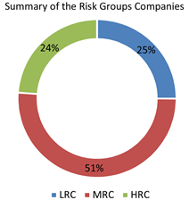
Table 7 provides a summary of the risk categorization in the Turkish manufacturing sector, presenting cumulative weighted average values over the observed period: Low Risk at 25%, Moderate Risk at 51%, and High Risk at 24%. These averages reveal that, across the timeframe, most companies fell into the moderate-risk category, followed by low-risk and high-risk categories.

The Turkish production and manufacturing sector has navigated through a range of unique challenges, including fluctuations in global demand, technological shifts, and intense competition, all of which have potential implications for financial stability and risk categorization. The sector’s financial profiles were significantly influenced by Türkiye’s dynamic economic policies, market conditions, government interventions, inflation rates, currency volatility, and trade dynamics (Utku-Ismihan & Pamukçu, 2020) .

Furthermore, comparing the risk categorization within the Turkish manufacturing sector to global trends during the same period could yield additional insights. External factors such as global economic downturns, trade disputes, and international conflicts might have indirectly impacted the sector. Additionally, the pandemic’s profound effect on global business operations, including supply chain disruptions, shifts in consumer behavior, and economic uncertainties, likely contributed to the observed fluctuations in risk categories, particularly the increase in high-risk companies.

Table 7. Summary of the risk categorization.

In essence, this analysis paints a picture of a dynamically evolving risk landscape within the Turkish manufacturing sector. The proportions of companies across different risk categories have shifted over time, influenced by a combination of internal factors and external events such as economic policies, geopolitical developments, and the pandemic. These influences have played a critical role in shaping the financial health and risk profiles of companies in the sector.

5.3.4. Impact of Non-Audited Reports on Financial Risk Assessment

Table 6 clearly showed significant fluctuations in the risk categories, particularly from the third to the fourth quarter of each year spanning 34 quarters from the first quarter of 2023 to the fourth quarter of 2014. This pattern could be attributed to the difference in reporting requirements for the Turkish stock exchange authority, where only the fourth quarter (year-end) reports are required to be externally audited.

Non-audited financial statements for the first three quarters introduced a higher degree of uncertainty in the financial data, as they lacked the scrutiny and validation that come with an external audit. This can lead to increased volatility in risk assessments. Without the rigor of an external audit, there is a higher potential for financial anomalies in the reported figures. The audited fourth-quarter reports are critical for a more accurate assessment of creditworthiness. They provide a corrective mechanism to earlier estimations based on non-audited data.

The fourth quarter often included year-end financial statements, which provided a comprehensive view of a company’s annual performance. Significant changes in risk categories during this period reflected adjustments based on the full year’s data. Therefore, the fourth-quarter reports, being audited, are likely to present a more accurate and reliable picture of a company’s financial health. The introduction of audited data has led to significant adjustments in risk categorization, explaining the observed volatility.

Furthermore, fluctuations in risk categories due to non-audited reports have led to temporary misalignments in a company’s perceived creditworthiness. Investors and creditors observed a shift in a company’s risk profile with the release of audited fourth-quarter reports. Regarding strategic considerations for companies, they managed their performance differently across quarters, knowing the audit requirements. This involved strategic financial decisions that impact quarterly reporting. The pattern of volatility has been anticipated by investors, leading to adjusted expectations and investment strategies based on the timing of audited information.

In conclusion, the pronounced quarterly variations in risk categorizations, especially the marked changes in Q4, emphasized the crucial role of audited financial statements in accurate financial risk and creditworthiness assessment. This trend underscored the challenges of relying solely on non-audited financial data and highlighted the audited reports’ role in providing a clearer, more reliable picture of a company’s financial health. Thus, external stakeholders should interpret financial data cautiously across quarters, placing greater emphasis on comprehensive, audited year-end financial statements.

5.4. Influential Financial Ratios

Throughout this study, the Mahalanobis Distance has been instrumental in detecting financial outliers and anomalies, pivotal in assessing financial risks and validating the accuracy of financial data. Additionally, the incorporation of feature importance analysis and dimensionality reduction techniques like Principal Component Analysis (PCA) has proven vital. These techniques refine the anomaly detection model’s precision and unveil deeper insights into financial data, thus enhancing the robustness and depth of our analysis. The integration of PCA with Mahalanobis distance forms a robust method for identifying anomalies in complex, high-dimensional financial datasets, essential for discerning financial risks and ensuring the integrity of financial data.

A critical aspect of this research involves understanding which financial ratios significantly impact anomaly prediction. With 34 different variables (financial ratios) comprising our high-dimensional dataset, PCA was employed to simplify this data while preserving its variability.

Using Python’s scikit-learn library, PCA was applied to these 34 financial ratios. The explained variance ratio for each component was computed, showcasing the PCA algorithm’s efficacy in managing complex calculations. This process included data standardization, covariance matrix computation, Eigen decomposition (key to understanding the principal components) and selecting principal components in descending order of importance.

Table 8 presents the results of the PCA analysis, including component loadings that indicate each financial ratio’s contribution to the principal components. These loadings, detailed across 34 rows corresponding to financial ratios,

Table 8. Principal Component Analysis (PCA).

are associated with 21 principal components (PCs) in the “PC” columns of the Excel file. This analysis guided the selection of an optimal number of components based on the cumulative explained variance. By analyzing the component loadings, we determined the significance of each financial ratio in these components. We chose 21 principal components that collectively account for at least 85% of the total variance in the dataset. This balance between information retention and feature reduction is critical for effective financial analysis and risk assessment.

5.4.1. The Most Influential Financial Ratios in the PCA

The contribution of key financial ratios to the variance captured by the principal components in our PCA analysis. This detailed breakdown as presented in Table 8 is instrumental for enhancing our understanding of anomaly detection within financial statements.

The PCA prioritized specific financial ratios based on their impact on the variability in the dataset. It highlighted “R24” (Asset Profitability), “R27” (EBITDA to Total Debts), “R9” (Short-Term Debt to Current Assets), “R19” (Net Sales to Short-Term Debts), and “R1” (Current Ratio) as the most influential ratios. Remarkably, these ratios consistently emerge as top contributors across various principal components.

Figure 4 visually represents the influence of these five financial ratios on the first 21 principal components. Each line in the figure signifies a financial ratio, with the loading factor on the y-axis indicating the strength and direction of the ratio’s association with each principal component.

This analysis of influential financial ratios is pivotal in financial scrutiny. Understanding their significance in the broader context of financial analysis offers deep insights into potential anomalies, risks, and managerial inefficiencies in corporate financial statements. These ratios, by virtue of their influence on the principal components, provide a focused lens through which to examine the financial health and stability of companies in the dataset.

Asset Profitability:

Briefly starting with the most influential financial ratio, asset profitability, in the principal component analysis (PCA), it has a strong loading across multiple components, suggesting it’s a key driver of variance among the ratios. It measures the return on total assets, assessing a firm’s ability to generate profits from its assets. The ratio shows the highest variability in PCA. it means that this ratio significantly differs across companies in the dataset and contributes greatly to the variance captured by the principal components. This implies that Asset Profitability is a key metric in differentiating the financial health and operational efficiency of companies in this analysis.

The high variability of Asset Profitability in PCA makes it a crucial metric for spotting financial anomalies. Significant deviations from typical industry ratios or historical trends can indicate operational issues or financial irregularities. For example, unusually high asset profitability could suggest overly aggressive

Figure 4. Most influential financial ratios.

accounting practices or a particularly effective business model, whereas unusually low profitability might signal inefficiencies, underutilization of assets, or deeper financial problems. Hence, Asset Profitability, with its high variability in PCA, emerges as a critical factor in distinguishing between companies’ financial profiles. Its analysis is essential for understanding how effectively a company is using its assets to generate profits and for detecting potential operational inefficiencies or financial anomalies.

EBITDA to Total Debts:

EBITDA to Total Debts reflects the earning capacity of a company in relation to its total debts. Given its second high variability and impact in PCA, this ratio is particularly useful in detecting financial anomalies. This means that EBITDA to Total Debts is a key factor in differentiating the financial profiles of companies, making it highly influential in the analysis. Significant deviations from industry norms or historical averages in this ratio could signal financial distress or an unsustainable debt structure. The ratio indicates that the company is not generating sufficient earnings to cover its debt obligations, possibly leading to liquidity issues. A very high ratio is also a sign of underleverage for a company facing difficulties borrowing or mobilizing on-balance-sheet resources from the market due to its lack of creditworthiness. Thus, the EBITDA to Total Debts ratio’s significant variability and impact in PCA analysis make it a vital tool for financial risk assessment. Its effectiveness in identifying variations in debt management and operational profitability is crucial for determining the financial health of companies within the dataset.

Short-Term Debt to Current Assets:

This ratio emerged as the third most influential financial ratio. This ratio is an essential liquidity measure, indicating a company’s ability to cover its short-term obligations with its most liquid assets. Its importance in PCA underlines the significant variability of this ratio across different companies in our dataset, which markedly contributes to the overall variability in financial health, especially concerning liquidity. A high Short-Term Debt to Current Assets ratio signals potential liquidity issues, suggesting that a company may struggle to meet its short-term debts. On the flip side, a lower ratio implies stronger liquidity and overall financial stability. The substantial variability of this ratio in PCA analysis indicates its pivotal role in differentiating companies based on their financial health, particularly in terms of liquidity management.

Given its pronounced variability in PCA, this ratio is particularly crucial for identifying financial anomalies. Large deviations from industry standards or historical trends could point to financial instability, mismanagement, or an elevated level of risk-taking in liquidity management. For instance, a significantly high Short-Term Debt to Current Assets ratio may be indicative of impending financial distress or poor liquidity management practices. Conversely, an extremely low ratio might suggest a potential underutilization of available resources or excessively conservative financial strategies. Therefore, this ratio, with its high variability in PCA, emerges as a crucial metric for assessing a company’s liquidity and short-term financial health as well as its overall creditworthiness. Its analysis is essential for understanding how well a company can meet its short-term obligations and for identifying potential liquidity issues or financial anomalies.

Net Sales to Short-Term Debts:

The Net Sales to Short-Term Debts ratio, which measures a company’s efficiency in generating sales revenue against its short-term financial obligations, serves as a key indicator of operational efficiency and liquidity. The pronounced variability of this ratio in PCA highlights its importance in detecting financial anomalies. Deviations from established industry norms or historical trends in this ratio can signal financial distress or irregularities in operations. For example, an unusually high ratio might suggest over-reliance on sales for covering short-term debts or aggressive revenue recognition practices. On the other hand, an exceptionally low ratio could indicate operational issues, a decline in sales, or an increase in debt levels.

Notable discrepancies in this ratio can reveal underlying financial vulnerabilities, essential for evaluating a company’s overall credit risk. Therefore, this ratio emerges as a critical tool in the early detection of financial anomalies and assessment of financial stability, providing vital insights for stakeholders concerned with a company’s fiscal health.

Current Ratio:

In this analysis, the current ratio emerged as a critical financial metric, playing a significant role in differentiating the financial profiles of companies, particularly in terms of liquidity. The ratio measures a company’s ability to cover its short-term liabilities with its short-term assets. This ratio is indispensable for assessing a company’s short-term financial health, underlining its capability to meet immediate obligations with assets that can be quickly converted into cash. The prominence of the current ratio within the PCA underscores its importance in identifying financial anomalies. Notably, unusual variations in this ratio may signal financial instability, potential mismanagement, or even looming solvency issues. For instance, a declining current ratio may indicate rising liabilities or diminishing assets, acting as early warning signs of financial distress.

The analysis of the current ratio’s fluctuations is crucial in understanding a company’s liquidity management. Sharp changes in this ratio can reveal underlying issues in cash flow management or operational efficiency. In the broader context of financial risk assessment, the Current Ratio serves as a key indicator, providing insights into a company’s ability to maintain financial equilibrium in the short term. Its relevance in the PCA analysis demonstrates its utility as a diagnostic tool in financial analysis, offering a reliable measure for evaluating corporate financial health and stability.

In brief, identification of these key ratios through PCA provided a focused lens for detecting financial anomalies. These ratios, by virtue of their influence on the variance in the dataset, are crucial indicators of a company’s financial health and are instrumental in highlighting potential areas of concern, be it from operational inefficiencies, financial distress, or even fraudulent activities. Understanding and monitoring these ratios closely can significantly support the early detection of financial irregularities.

Ratios related to liquidity, debt, and profitability are crucial for Turkish companies, especially given the currency fluctuations and inflation. For instance, ratios indicating short-term liquidity such as the current ratio or debt obligations like EBITDA to Total Debts would be important in assessing the resilience of businesses during economic fluctuations.

5.4.2. The Least Influential Financial Ratios in the PCA

Understanding the least influential financial ratios in Principal Component Analysis (PCA) is crucial, particularly when aiming to capture the complete array of factors impacting a financial dataset. In our analysis, certain financial ratios exhibited low variability, indicating their limited influence in differentiating companies based on their financial profiles. These ratios are less associated with financial anomalies or irregularities, suggesting areas that might be less critical to the dataset’s overall variability or specific outcomes like anomaly prediction.

Low variability in these financial ratios implies that they do not vary significantly across different companies and, therefore, do not contribute substantially to the principal components. Such limited variation suggests that these ratios are not the key differentiators in the financial profiles within the dataset under examination. This stability or consistency across observations indicated that these ratios are less indicative of financial distress or operational inefficiencies and could represent aspects of a company’s financial health that are generally sound.

Among the first five principal components, the ratios with the smallest absolute loadings, and thus the least influence, included “R14” (Net Working Capital Turnover), “R18” (Operating Expenses to Average Assets), “R34” (Market Value to EBITDA), “R17” (Efficiency Ratio/Assets Turnover Ratio), and “R31” (Change in Depreciation Expenses Ratio). These ratios consistently showed minimal contribution to the variance captured by these components.

Net Working Capital Turnover:

In this analysis for Turkish companies, especially during the COVID-19 period, the “Net Working Capital Turnover” surfaced as one of the least impactful financial ratios. This metric, which assesses a company’s efficiency in using its working capital to generate sales, was calculated by dividing Sales by net working capital. Its minimal variability in the PCA suggested that this ratio exhibited relatively uniform behavior across the companies in the dataset, thus contributing less to the overall variance in the data. Consequently, it was not a decisive factor in differentiating between the financial health or operational efficiency of the companies in this analysis.

Understanding the implications of variations in the net working capital turnover ratio, even if it holds less sway in the PCA, is crucial for a comprehensive financial risk assessment. It provides nuanced insights into how effectively companies manage their working capital in relation to their sales performance, which is especially relevant in turbulent economic times like the COVID-19 pandemic.

Operating Expenses to Average Assets:

The ratio of Operating Expenses to Average Assets emerged as one of the least variable metrics. This ratio, crucial for assessing a company’s efficiency in using its assets to cover operating expenses, showed minimal variability among the companies in the dataset, suggesting its limited role in differentiating financial profiles within the analysis. This provides a nuanced view of a company’s operational efficiency and asset utilization, which are critical aspects of financial health. Its analysis could reveal hidden financial stresses or efficiencies in a company’s operations, offering valuable insights into its financial management practices.

The low variability of this ratio in PCA implied that it is not a key determinant in distinguishing the diverse financial health of companies. However, its relevance in financial analysis should not be underestimated, particularly in identifying financial anomalies. A sudden increase in this ratio could indicate operational inefficiencies or rising operating expenses, which might not be evident through other financial metrics. Conversely, an unusually low ratio could raise concerns about the sustainability of such efficiencies or potential under-reporting of expenses or over-valuation of assets, potentially pointing to financial manipulation.

Market Value to EBITDA:

This ratio emerged as one of the least influential financial ratios in terms of contributing to the overall variability. This ratio, which links a company’s market value to its earnings before interest, taxes, depreciation, and amortization, offers insights into investor expectations and company valuation.

The minimal variability of the Market Value to EBITDA ratio in the PCA suggested that this metric did not exhibit significant fluctuations across the dataset. Consequently, it contributed less to the variance explained by the principal components and was not a primary determinant in differentiating the financial profiles of companies within this study. However, despite its reduced influence in the PCA, the Market Value to EBITDA ratio holds importance in identifying financial anomalies. For instance, an abnormally high Market Value to EBITDA ratio might signal overvaluation, potentially indicative of a market bubble or excessively optimistic investor expectations. Conversely, a very low ratio could point to undervaluation, possibly due to overlooked positive company attributes or general market pessimism. Therefore, while the Market Value to EBITDA ratio may not be a key factor in the PCA’s variability, it remains a valuable metric for financial analysis, particularly in evaluating market perception and investment trends.

Efficiency Ratio:

Certain financial ratios exhibited less influence on the variability of the data, with the efficiency ratio being another notable example. This ratio, more commonly pertinent to the banking or finance sector, demonstrated limited applicability and impact in the context of the manufacturing industry within our study. Consequently, it ranked relatively lower in terms of its influence in the PCA.

A stable or consistent efficiency ratio indicates operational effectiveness, reduced operating costs, or steady income generation. In the broader scope of financial analysis, this ratio serves as an indicator of a company’s resource utilization efficacy. However, its lower significance in the PCA for our study highlights the varying impact and relevance of financial ratios across different industries. Further, the lower influence of the efficiency ratio in the PCA emphasizes the importance of sector-specific financial analysis. It indicates that while some financial ratios are universally applicable, others may have limited relevance outside their primary industry context.

Change in Depreciation Expenses:

Lastly, this estimated as another less influential financial metrics. This ratio is utilized to assess the fluctuations in a company’s depreciation expenses over time. Depreciation, as an accounting concept, involves the systematic allocation of the cost of tangible assets over their useful life. It accounts for factors such as wear and tear, obsolescence, or other forms of value depreciation over time.

The PCA analysis revealed that variations in the “depreciation expenses ratio” were relatively low, indicating its minimal impact in distinguishing among companies based on their financial profiles. However, this does not diminish its relevance in financial analysis. A substantial change in depreciation expenses could indicate new acquisitions, disposals of assets, or changes in depreciation methods, each of which has implications for a company’s financial health and strategy. Therefore, in comprehensive financial risk assessments, attention should be given to the ratio, especially when it deviates markedly from expected values.

In short, each of the financial ratios serves distinct purposes in financial analysis but demonstrates low variability in the PCA, suggesting they are not primary differentiators in a dataset. Despite their lower impact in PCA, these ratios are crucial for detecting financial anomalies and understanding a company’s financial health, offering insights into operational efficiency, asset management, and valuation discrepancies in the context of industry norms and historical performance. Thus, they could serve as foundational elements that support a company’s creditworthiness.

Moreover, identifying influential financial ratios in PCA can help in recognizing stable areas in a volatile economic environment. For Turkish companies, stability in certain financial metrics could signal robust business models or effective risk management strategies in a challenging economic landscape. while the most influential financial ratios in a PCA could draw more attention, especially in identifying potential anomalies or areas of significant variability, the least influential ratios are equally important in painting a complete picture of financial health. They can indicate areas of stability and reliability, which are essential components of a comprehensive credit risk assessment and overall financial analysis.

The economic perspective of Türkiye, particularly during the COVID-19 period, reflects a scenario of resilience amid challenges. Financial ratios and their analysis provide valuable insights into the health and stability of Turkish companies and the economy. Understanding both the most and least influential ratios in this context can offer a comprehensive view of the financial impacts of the pandemic, as well as the underlying strengths and weaknesses of the Turkish economy.

5.5. Contribution to the Research Gap

This research thoroughly explores the intricate dynamics of financial ratios, pinpointing anomalies and evaluating their influence on the credit quality of companies in the production and manufacturing sectors listed on the Istanbul Stock Exchange. It significantly contributes to the domain of financial analytics in these sectors by offering comprehensive insights into the role of financial ratios in creditworthiness assessment. This study fills a notable research gap by being the first to combine dimensionality reduction techniques, specifically principal component analysis (PCA), with the Mahalanobis distance. This new integration not only enhances the model for anomaly detection but also contributes to the field of financial analytics in these sectors.

Using Python-driven machine learning, the study scrutinizes data from 254 companies over 2014-2023. It was discovered that 89.61% of cases are normal, falling into low or moderate risk categories, while 10.39% are anomalies, indicating high risk. This implies a predominant consistency in financial indices among a significant number of companies. Moreover, the study reveals significant fluctuations in risk categorization, particularly in the second half of each year, which may reflect differences in reporting and auditing practices. Through PCA, key financial ratios such as asset profitability and EBITDA to total debts were identified as highly influential, while others like net working capital turnover showed lesser impact. This innovative combination of PCA and Mahalanobis distance is a pioneering approach in the field, offering a new perspective and narrowing the research gap in financial analytics, particularly in the context of detecting financial anomalies and assessing creditworthiness.

6. Conclusion

This study presents a comprehensive analysis of financial ratio anomalies and their implications on the creditworthiness of companies listed on the Istanbul Stock Exchange (ISE), specifically focusing on the production and manufacturing sectors. The distinctiveness of this research lies in its methodological approach, which combines Python-driven machine learning techniques with the Mahalanobis distance to identify and interpret financial ratio anomalies.

The analysis period, spanning from the fourth quarter of 2014 to the first quarter of 2023, involved a thorough examination of financial data from 254 companies. This provided insights into the evolving economic landscape and its impact on corporate financial health. As a result of applying the Mahalanobis distance, 89.61% of observations were classified as normal, and 10.39% were classified as anomalies. This suggests that a significant majority of the companies have financial indices within expected ranges.

Despite the seemingly small anomaly rate of 10.39%, in the context of 189,000 observations, this constitutes a considerable number of data points (approximately 19,637 observations) that are markedly different from the norm. These anomalies could stem from extraordinary financial conditions, potential financial distress, reporting errors, or irregularities, marking these companies as high financial risk. The model’s performance evaluation revealed excellent precision and a perfect ROC-AUC score, demonstrating its excellent capability in distinguishing between the classes of anomalies and non-anomalies. However, the model exhibited a moderate recall, indicating room for improvement in capturing more true anomalies.

Companies were further categorized into different risk tiers such as “Low Risk,” “Moderate Risk,” or “High Risk,” based on their Mahalanobis distances. These classifications were made commensurate with the data points considered as anomalies, with chosen thresholds leading to a distribution of low risk at 25%, moderate risk at 51%, and high risk at 24%, based on the cumulative weighted average values across the period. These averages suggest that most companies were categorized as low-risk and moderate-risk, followed by high-risk categories during the observed period.

Significant fluctuations in risk categories were observed, particularly from the third to the fourth quarter of each year, spanning 34 quarters from the first quarter of 2014 to the fourth quarter of 2023. This fluctuation is attributed to differences in reporting requirements by the authority, where only year-end reports in the fourth quarter are mandated to be audited.

A fundamental aspect of this study was the implementation of feature importance analysis and the application of dimensionality reduction techniques, notably Principal Component Analysis (PCA). After ranking the financial ratios based on their importance, PCA analysis identified “Asset Profitability,” “EBITDA to Total Debts,” “Short-Term Debt to Current Assets,” “Net Sales to Short-Term Debts,” and “Current Ratio” as the most influential financial ratios. These ratios are significant indicators of potential anomalies, risks, and mismanagement in a company’s financial statements.

Conversely, identifying the least influential financial ratios in PCA, based on the smallest absolute loadings, is equally important. These include “Net Working Capital Turnover,” “Operating Expenses to Average Assets,” “Market Value to EBITDA,” “Efficiency Ratio (Assets Turnover Ratio),” and “Change in Depreciation Expenses Ratio (annual difference in depreciation expense),” indicating their lower impact in PCA and their lesser role in differentiating financial anomalies. Despite their lower impact in PCA, these ratios are crucial for understanding their minimal contributions to financial anomalies and a company’s financial health within the context of industry norms and historical performance, serving as foundational elements in evaluating a company’s creditworthiness.

In essence, the core findings of this research underscore the multifaceted nature of financial anomalies within Turkish industries. The application of Mahalanobis distance, coupled with dimensionality reduction techniques like PCA, has revealed subtle yet significant deviations in financial ratios, often obscured in traditional analyses. These anomalies, while not direct indicators of fraudulent activities, are essential red flags for evaluating creditworthiness. The methodological innovation of this study lies in its ability to quantify the severity of these anomalies and correlate them with the fluctuating credit quality of companies on a quarterly basis.

7. Challenges and Limitations

While pioneering in its approach, this study encounters several challenges and limitations in assessing the financial anomalies and creditworthiness of ISE-listed companies.

A primary limitation of this study is the nature of the data itself. The financial data of ISE-listed companies, though extensive, may not fully encapsulate the dynamic nature of financial markets or the intricacies of individual company operations. Potential biases in the data may arise due to several factors, including incomplete reporting, divergent accounting practices among companies, or the inherently historical nature of financial data, which may not reliably forecast future trends. As highlighted in the previous section, the reporting requirements mandated by authorities, specifically the stipulation for auditing only the year-end reports in the fourth quarter, could introduce biases in the dataset (Suryono, Budi, & Purwandari, 2020) .

Regarding external factors, they significantly influence the financial health and creditworthiness of companies. Elements like macroeconomic changes, regulatory shifts, and market dynamics could substantially affect financial anomalies but are not directly accounted for in this analysis. Global economic fluctuations or sector-specific regulatory changes, for instance, might profoundly impact the creditworthiness of these companies, factors that our model may not have fully captured (Johnson, 2020) .

Applying machine learning techniques to financial data presents unique challenges. The complexity and variability of financial data often necessitate sophisticated preprocessing to ensure data quality and relevance. The Mahalanobis Distance, a robust statistical tool, requires careful calibration and validation when applied in a machine learning context. This is particularly challenging when handling the high dimensionality and multicollinearity often present in financial datasets. Additionally, the predictive accuracy of the model can be affected by overfitting, a common issue when dealing with limited dataset sizes, as is often the case in specific sectors like production and manufacturing (Brown, 2019) . Thus, while this study provides valuable insights into financial anomalies and creditworthiness using an advanced machine learning approach, it is important to acknowledge these challenges and limitations.

Conflicts of Interest

The author declares no conflicts of interest regarding the publication of this paper.

References

[1]	Agrawal, A., & Cooper, T. (2017). Corporate Governance Consequences of Accounting Scandals: Evidence from Top Management, CFO and Auditor Turnover. The Quarterly Journal of Finance, 7, Article 1650014. https://doi.org/10.2139/ssrn.970355
[2]	Allwright, S. (2022). How to Interpret AUC Score? https://stephenallwright.com
[3]	Altman, E. I. (1968). Financial Ratios, Discriminant Analysis and the Prediction of Corporate Bankruptcy. The Journal of Finance, 23, 589-609. https://doi.org/10.1111/j.1540-6261.1968.tb00843.x
[4]	Atiyas, I. (2013). Think Tank 20: The G-20 and Central Banks in the New World of Unconventional Monetary Policy. Brookings.
[5]	Barboza, F., Kimura, H., & Altman, E. (2017). Machine Learning Models and Bankruptcy Prediction. Expert Systems with Applications, 83, 405-417. https://doi.org/10.1016/j.eswa.2017.04.006
[6]	Beaver, W. H. (1968). Market Prices, Financial Ratios, and the Prediction of Failure. Journal of Accounting Research, 6, 179-192. https://doi.org/10.2307/2490233
[7]	Berument, H., & Taşçı, H. (2002). Inflationary Effect of Crude Oil Prices in Turkey. Physica A: Statistical Mechanics and its Applications, 316, 568-580. https://doi.org/10.1016/S0378-4371(02)01025-7
[8]	Bigan, I., Decan, S., & Korkmaz, B. (2017). How Turkish Companies Can Become Global Successes. McKinsey & Company. Perspectives on Retail and Consumer Goods, No. 6. https://www.mckinsey.com/~/media/McKinsey/Industries/Retail/Our%20Insights/How%20Turkish%20companies%20can%20become%20global%20successes/How-Turkish-companies-can-become-global-successes.pdf
[9]	Brealey, R., Myers, S., & Allen, F. (2020). Principles of Corporate Finance. McGraw-Hill Education.
[10]	Brown, R. (2019). Machine Learning in Finance: Opportunities and Risks. AI and Finance, 2, 45-60.
[11]	Davis, J. S., & Pesch, H. L. (2013). Fraud Dynamics and Controls in Organizations. Accounting, Organizations and Society, 38, 469-483. https://doi.org/10.1016/j.aos.2012.07.005
[12]	Deakin, E. B. (1972). A Discriminant Analysis of Predictors of Business Failure. Journal of Accounting Research, 10, 167-179. https://doi.org/10.2307/2490225
[13]	Demir, E., & Gök, B. (2018). Bankruptcy Prediction Using Diverse Machine Learning Algorithms. In 2018 6th International Conference on Future Internet of Things and Cloud Workshops (FiCloudW) (pp. 1-6). IEEE.
[14]	Erdogdu, E. (2007). Regulatory Reform in Turkish Energy Industry: An Analysis. Energy Policy, 35, 984-993. https://doi.org/10.1016/j.enpol.2006.02.011
[15]	Ertuğrul, İ., & Karakaşoğlu, N. (2009). Performance Evaluation of Turkish Cement Firms with Fuzzy Analytic Hierarchy Process and TOPSIS Methods. Expert Systems with Applications, 36, 702-715. https://doi.org/10.1016/j.eswa.2007.10.014
[16]	European Bank for Reconstruction and Development (EBRD) (2021). Turkey: Manufacturing Resilience Programme. EBRD.
[17]	Giannopoulos, G., & Sigbjørnsen, S. (2019). Prediction of Bankruptcy Using Financial Ratios in the Greek Market. Theoretical Economics Letters, 9, 1114-1128. https://doi.org/10.4236/tel.[phone]
[18]	Gönenç, H., Karpat-Çatalbaş, G., & Biçerli, M. K. (2019). Sectoral Analysis of Financial Ratios: A Panel Data Approach. International Journal of Economics and Financial Issues, 4, 1-10.
[19]	Hawkins, D. M. (1980). Identification of Outliers (Vol. 11). Chapman and Hall. https://doi.org/10.1007/978-94-015-3994-4
[20]	International Trade Administration. (2021). Turkey-Energy.
[21]	Jia, W., Sun, M., Lian, J., & Hou, S. (2022). Feature Dimensionality Reduction: A Review. Complex & Intelligent Systems, 8, 2663-2693. https://doi.org/10.1007/s40747-021-00637-x
[22]	Johnson, L. (2020). Macroeconomic Influences on Financial Markets. Global Economics Review, 89-103.
[23]	Jones, S. (2023). A Literature Survey of Corporate Failure Prediction Models. Journal of Accounting Literature, 45, 364-405. https://doi.org/10.1108/JAL-08-2022-0086
[24]	Kamoi, R., & Kobayashi, K. (2020). Why Is the Mahalanobis Distance Effective for Anomaly Detection? arXiv preprint arXiv:2003.00402
[25]	Kazgan, G. (2012). Dünden bugüne küreselleşmenin ekonomik temelleri (No. 2012/53). Discussion Paper.
[26]	Kepenek, Y., & Yentürk, N. (2005). Türkiye Ekonomisi. Remzi Kitabevi (12. Baskı).
[27]	Kumar, B. S., & Ravi, V. (2016). A Survey of the Applications of Text Mining in the Financial Domain. Knowledge-Based Systems, 114, 128-147. https://doi.org/10.1016/j.knosys.2016.10.003
[28]	Liu, Z., Huang, D., Huang, K., Li, Z., & Zhao, J. (2021). Finbert: A Pre-Trained Financial Language Representation Model for Financial Text Mining. In C. Bessiere, (Ed.), Proceedings of the Twenty-Ninth International Conference on International Joint Conferences on Artificial Intelligence (pp. 4513-4519). International Joint Conferences on Artificial Intelligence. https://doi.org/10.24963/ijcai.2020/622
[29]	Lokanan, M., Tran, V., & Vuong, N.H. (2019). Detecting Anomalies in Financial Statements Using Machine Learning Algorithm: The Case of Vietnamese Listed Firms. Asian Journal of Accounting Research, 4, 181-201. https://doi.org/10.1108/AJAR-09-2018-0032
[30]	Markopoulos, A. P., Perakis, M., Valavanis, K. P., & Rassias, T. M. (2015). A DEA Approach for Estimating the Efficiency of Manufacturing and Agricultural Companies. Journal of Computational and Applied Mathematics, 290, 264-275.
[31]	Mehmet, O., & Yorucu, V. (2021). Modern Geopolitics of Eastern Mediterranean Hydrocarbons in an Age of Energy Transformation. Insight Turkey, 23, 294-297. https://doi.org/10.1007/978-3-030-43585-1
[32]	Öğüt, H., Doğanay, M. M., Ceylan, N. B., & Aktaş, R. (2012). Predicting Bank Financial Strength Ratings: The Case of Turkey. Economic Modelling, 29, 632-640. https://doi.org/10.1016/j.econmod.2012.01.010
[33]	Öniş, Z., & Webb, S. B. (1992). Political Economy of Policy Reform in Turkey in the 1980s (Vol. 1059). World Bank Publications.
[34]	Republic of Türkiye Ministry of Energy and Natural Resources (2020). Energy Efficiency Action Plan 2019. https://enerji.enerji.gov.tr/Media/Dizin/EVCED/tr/Raporlar/NEEAP_Progress_Report_2019.pdf
[35]	Ross, S., Westerfield, R., & Jordan, B. (2019). Essentials of Corporate Finance. McGraw-Hill Education.
[36]	Siami-Namini, S., Tavakoli, N., & Siami Namin, A. (2018). A Comparison of ARIMA and LSTM in Forecasting time Series. In 2018 17th IEEE International Conference on Machine Learning and Applications (ICMLA) (pp. 1394-1401). https://doi.org/10.1109/ICMLA.2018.00227
[37]	Stöckl, S., & Hanke, M. (2014). Financial Applications of the Mahalanobis Distance. Applied Economics and Finance, 1, 78-84. https://doi.org/10.11114/aef.v1i2.511
[38]	Suryono, R. R., Budi, I., & Purwandari, B. (2020). Challenges and Trends of Financial Technology (Fintech): A Systematic Literature Review. Information, 11, Article 590. https://doi.org/10.3390/info11120590
[39]	Tarim, S. A., & Karan, M. B. (2001). Investment Fund Performance Measurement Using Weight-Restricted Data Envelopment Analysis: An Application to the Turkish Capital Market. Russian & East European Finance and Trade, 37, 64-84.
[40]	The International Energy Agency (IEA) (2020). Turkey 2020: Energy Policy Review. https://www.iea.org/reports/turkey-2020
[41]	Tripathi, D., Edla, D.R., & Bablani, A. (2021). Experimental Analysis of Machine Learning Methods for Credit Score Classification. Progress in Artificial Intelligence, 10, 217-243. https://doi.org/10.1007/s13748-021-00238-2
[42]	Trivedi, S. K. (2020). A Study on Credit Scoring Modeling with Different Feature Selection and Machine Learning Approaches. Technology in Society, 63, Article 101413. https://doi.org/10.1016/j.techsoc.2020.101413
[43]	Turkish Statistical Institute (2022). Manufacturing Industry Statistics. Turkish Statistical Institute. http://www.turkstat.gov.tr/PreTablo.do?alt_id=1022
[44]	Utku-Ismihan, F. M., & Pamukçu, M. T. (2020). Determinants of Growth Performance of High Growth Firms: An Analysis of the Turkish Manufacturing Sector. Economic Research Forum (ERF).
[45]	Wang, H., & Zheng, H. (2013). Model Testing, Machine Learning. In W. Dubitzky, O. Wolkenhauer, K. H. Cho, & H. Yokota (Eds.), Encyclopedia of Systems Biology (p. 1405). Springer. https://doi.org/10.1007/978-1-4419-9863-7_231
[46]	Wang, J., Sun, T., Liu, B., Cao, Y., & Wang, D. (2018). Financial Markets Prediction with Deep Learning. In 2018 17th IEEE International Conference on Machine Learning and Applications (ICMLA) (pp. 97-104). IEEE. https://doi.org/10.1109/ICMLA.2018.00022
[47]	Wang, J., Sun, T., Liu, B., Cao, Y., & Wang, D. (2020). Mahalanobis Distance Based Adversarial Network for Anomaly Detection. In ICASSP 2020-2020 IEEE International Conference on Acoustics, Speech and Signal Processing (ICASSP) (pp. 3317-3321). IEEE.
[48]	Wasserbacher, H., & Spindler, M. (2022). Machine Learning for Financial Forecasting, Planning and Analysis: Recent Developments and Pitfalls. Digital Finance, 4, 63-88. https://doi.org/10.1007/s42521-021-00046-2
[49]	Yang, S., & Gui, Z. (2023). An Introduction on the Multivariate Normal-Ratio Distribution. arXiv preprint arXiv:2310.14306
[50]	Zhang, Z., Cheng, Y., & Liu, N. C. (2014). Comparison of the Effect of Mean-Based Method and Z-Score for Field Normalization of Citations at the Level of Web of Science Subject Categories. Scientometrics, 101, 2129-2140. https://doi.org/10.1007/s11192-014-1294-7