How Users Perceive Infrastructure Development Affects Their Transport Mode Choice

Lina Shbeeb

Civil Engineering Department, Hussein Technical University, Amman, Jordan.

DOI: 10.4236/jtts.2023.134025                

Abstract

Transport infrastructure development and perception vary across and within countries, influencing mode choice among road users. This study explores how road users perceive the development of infrastructure modes, service attributes, embedded safety levels, and commuting modes. Additionally, the research examines whether participants’ environmental backgrounds impact their mode choice patterns. The study gathered responses from 1169 participants residing in two regions of Amman, Jordan, each with distinct infrastructure development and population densities. Participants completed a standardized questionnaire, and several statistical techniques were employed for analysis. The findings revealed that facilities’ infrastructure attributes, development, and safety were assessed using three indices. Both participant groups perceived these indices differently on average. Residents of low population density areas with relatively developed infrastructure showed more consistent assessments, irrespective of their most frequently used mode of transportation, tending towards lower scores. Interestingly, subjective ratings of infrastructure development were higher (4.96) than attribute-based ratings (4.32). Despite their generally low-quality perception, public transportation services received the highest appraisal (4.9). Conversely, pedestrian infrastructure complementing public transport received the lowest assessment (4.57), only slightly higher than street environments (4.59). The study found weak associations between subjective service characteristics ratings. Traveler and trip characteristics influenced mode choice and trips more than infrastructure perception. In conclusion, the study suggests that policies should be developed to encourage green transportation, ensure social equality and safety. In addition, the study contributes to understanding perceptions about transport infrastructure, modes of transportation, and the factors that influence sustainable and equitable transportation systems.

Keywords

Road Index, Infrastructure Development, Infrastructure Attribute, Safety Rating, Structural Equation Models, Modal Choice

1. Introduction

The 2021 budget of Greater Amman municipality shows that 10% of its expenditures go to developing the city infrastructure, such as asphalt, aggregate base and sub-base courses, ditches, culverts, and retaining walls. Last on the list was sidewalk work, even though one-quarter of all trips in Amman involve walking. Compared to public transportation, private cars make up one-third of all trips [1] . The Public Transport budget does not exceed 2%, except for the Bus Rapid Transit (BRT) project, which includes traffic enhancement components in 8% [2] . Public transport modal shares of 8% for buses and 5% for taxi-sharing services (white taxis) necessitate the development of the city’s BRT project [1] . While the public may not see the benefits associated with the new service, they still prefer reducing congestion and improving the car traffic environment. The modal choice factors include the perception of infrastructure, needs and desires, and affordability, which may contradict each other. The literature extensively discusses the modal choice and related factors at the individual level and includes service attributes describing the trip or exclusively for each mode. Public transportation is significantly affected by car ownership, distance to work, parking availability, and ticket prices as a daily commute mode in Norway and is negatively affected by low bus frequency and long walking distances to the home bus stop [3] . An ordered logit model for examining the impacts of perception of infrastructure on the use of shared space was developed using data from 200 face-to-face interviews from Palemero, Italy, indicating that perceptions of safety and comfort for walking and cycling increase with one-unit higher perceptions of infrastructure; the gender and age influence the use of the shared space [4] . A literature review of several studies was prepared in New Zealand to provide an overview of key infrastructure initiatives that provide a safe and healthy environment for active transportation; according to the study teams, mode choice is influenced by the quality and type of infrastructure users encounter on a trip-by-trip basis. The quality of infrastructure affects pedestrians’ and cyclists’ safety, safety perception, and overall service levels [5] . Travelers in five northern European cities were surveyed to validate the relationship between public transport quality and perceived accessibility and the role of perceived safety. Several factors affect the perceived quality of public transportation, including functionality (reliability, travel time, frequency, distance), information (reliable and timely), comfort (cleanliness and accessibility to seats), and cost (fare structure, tickets, and their validity). There is a direct correlation between perceived accessibility and functionality and an indirect with perceived travel safety, with some variations among the cities. There was an association between females’ age and gender and their perceptions of accessibility [6] .

To examine drivers’ perceptions and opinions of road infrastructure, trip characteristics, and daily trip experiences, researchers conducted a five-country study in Estonia, Greece, Kosovo, Russia, and Türkiye. They concluded that road users had very different perceptions and evaluations of environmental characteristics [7] . In the Lisbon metropolitan area, ethnographic interviews and focus group discussions were conducted to identify factors affecting people’s perceptions and satisfaction. According to Ramos et al. [8] a better intermodal connection, better compliance with timetables, and better response to the users’ needs will increase the use of public transportation. To provide policymakers with useful information on road transport infrastructure projects completed in cargo transportation in Brazil, a literature review was conducted. There are four most relevant variables: traveling time, atmospheric emissions, accident numbers, and operating costs, among others [9] . This online survey addressed the infrastructure service level assessment model based on citizen demand, highlighting the utility of the infrastructure index in setting priorities. The model evaluates usability (evidence that infrastructure functions properly), accessibility (accessibility when required), and disaster recovery speed. Residents’ satisfaction with their homes was significantly influenced by the quality of infrastructure in a residential area [10] .

Roads and public transportation are generally well-rated; men 46 - 55 gave the highest rating, while the youngest gave the lowest; men’s rating was usually higher than women. A high score was given to the readability of public transportation timetables, while the lowest score was given to accessibility and distribution. The study also found that bus stops and shared vehicles need to be safer, and parking spaces should be more plentiful [11] . In Greece, a probit model was developed to identify the variables affecting the modal choice for urban mobility; the study concluded that females and groups aged 35 - 44 prefer public transport. People don’t use public transportation mainly because of crowdedness, lack of information, and poor accessibility. By contrast, parking spaces would encourage the use of cars [12] .

The perception seems to be investigated as a synonym for satisfaction and its impact on mobility model selection without considering the other modes’ perceptions of the competing infrastructure. The perceptions of infrastructure usually are examined from one mode of transportation perspective, with few attempts to quantify it as a variable that may influence the user transport choice. The utility function discrete modal choice is derived from transport mode attributes that do not always include an indicator for user perception. Little research has been conducted on approaches and techniques for rating infrastructure in developing countries concentrating on one or more aspects. Government and community perspectives on existing and new infrastructure were investigated regarding their adequacy and perceptions [13] [14] . The studies aim to fill a gap in knowledge regarding the perception of infrastructure attributes, development, adequacy, safety, and their relation to modal choice.

As part of this study, road users’ perceptions of three modes of transportation were assessed separately and interrelatedly at the same time. First by evaluating the subject’s most frequent mode use; reflecting on other modes they are not primarily using. Secondly, by investigating whether modal choice is related to perception of mode attributes or, for other reasons, whether the users’ general perceptions of the development of transportation modes infrastructure are subjective or attributes-based perceptions based on budget allocated for development or other service attributes not related to infrastructure. In the end, the outcomes of this study will provide insight into policies that should be implemented to influence the perceptions and choices of users. To achieve the objectives of this study, the following hypotheses will be tested. Firstly, their socioeconomic status influences road users’ perceptions of transport infrastructure. Secondly, users assess the infrastructure of transportation modes they use for commuting similarly to modes they don’t (i.e., How their experience differed from their general perception). The third hypothesis, attribute-based users’ perceptions of transport infrastructure, is like their subjective perceptions. Fourthly, road users’ perception of infrastructure assessment is well correlated with attributes of infrastructure services, such as safety and stage of development. In the fifth hypothesis, the modal choice is not influenced by the user’s perception of modal characteristics. Two perspectives are considered to verify the last idea: individual choice and collective choice (aggregated level).

2. Literature Review

Traditionally, transport planning and policies focus on accessibility, mobility, and associated outcomes. Recently, the transport system design shifted from moving persons and goods to providing an affordable and safe system that serves everyone equally and efficiently [15] .

2.1. Transport Facilities’ Perception

Several studies investigated the user’s perception of the transport system. In Spain, a study showed that overall service quality was better explained when the passengers reflected on the service provided [16] . The perceived public transport accessibility, mobility, and seamless connectivity differ based on travellers’ age, frequency of weekly activities, and environmental awareness [17] . The causal pathway analysis investigated the link between the improvement of infrastructural intervention related to walking and cycling routes and behavior change, defined as the time spent walking and cycling. It indicated that user perception of improving new walking and cycling facilities in the UK was mainly because they were new routes. In contrast, pathways involving changes in environmental cognitions explained only a small proportion of the effect [18] . Based on a survey of 1221 participants, five European countries concluded that all road users (drivers’-motorcyclists, pedestrians, cyclists, and public transport) within and across the countries evaluated and perceived environmental facilities’ characteristics significantly differently [7] .

2.2. Transport Facilities’ Index

The land use and public transport accessibility index was a decision-aiding tool that used geographic system GIS-based methodology to quantify and map accessibility to common land use destinations by walking and public transport. It was applied on the Gold Coast of Queensland, Australia, to show how the accessibility indexing approach can be used as a decision-support tool in planning transportation and land-use activities [19] . Five methods were explored to develop composite road safety performance indicators. The weights derived from data envelopment analysis compared to the other four methods, factor analysis, analytic hierarchy process, budget allocation, and equal weighting, provided the highest correlation with the road safety ranking of 21 European countries based on the number of traffic fatalities per million inhabitants [20] . A street design index was created and validated through a testbed case study to address barriers to pedestrian access, crime fear, and broader social inclusion. Transport access for vulnerable groups is hindered by perceptions and safety concerns that need to be considered when planning mobility and journeys [21] .

A social-disadvantage index was used to identify neighborhoods needing attention during the review of the Montreal transportation plan, which was relatively equitable. However, some areas benefit greatly more than others. Still, the focus of most new transit infrastructure near the CBD, the plan does provide quite well for many poorer neighborhoods [22] . Later, the Montréal Origin-Destination survey conducted in 2003 examined the correlation of walkability scores with household travel behaviour for home-based trips. The study showed a correlation between walkability indices and walking trips for most non-work trip purposes, in addition to the role of socio-demographic characteristics on walking trips. Still, it was not the same for all individuals or households [23] .

2.3. Equity and Social Inclusion

According to the United Nations [24] , social inclusion is “the process of improving the terms of participation in society for disadvantaged people based on age, sex, disability, race, ethnicity, and economic and migration status”. Social inclusion and its relationship to the ability to be mobile and access opportunities were investigated. Public transport, including the emergence of autonomous public transport vehicles, might affect the options for reducing mobility-related social exclusion as potential means to support social inclusion [25] .

The equity and accessibility of the proposed transit infrastructure projects were also addressed, which showed that the plan was relatively equitable. However, some areas benefit much more than others on the regional and personal scales [22] . To address the accessibility inequality, different policies in Bogota related to changes in the fare structure of the existing public transport system and cross-subsidies used in appraising the impact of developing a new BRT line). The population, location, purchasing power, and a redistributive fare schemes market can be a more significant impact than the expansion and improvement of the public transport network on the accessibility to the labor market [26] . High public transport gaps characterize the suburban areas of the Dutch-speaking region of Belgium. These gaps differ over time when comparing the time-continuous and schedule-based public transport index to that based on the spatial distribution [27] . In Uruguay, unequal distribution of potential mobility was reported, especially for jobs and upper-level public education but not primary public schools [28] . The self-reported citizens’ needs were mapped with three urban transport policies in Port Louis city (Mauritius), including the light metro rail system, bus modernization scheme, and road decongestion program.

The citizen of Port Louis city, Mauritius, demanded improving sidewalks (80%), public spaces, green spaces, pedestrianizing strategic areas, centralizing street vendors at bus stations, and regulating the entry of private vehicles in the town. The study concluded that the policies aligned with three out of six needs of poorer population groups. At the same time, they do not respond to the need for the active mode of mobility, not addressing the health and social co-benefits of transport [29] . The impact of the accessibility to public transport on higher-quality public education was investigated. The results showed that around 20% of the zones in Santiago have at least a 50% deficit in higher-quality public education, and 71% are in peripheral areas classified as medium and low-income population areas where their transit passengers need, on average, 1 - 2 transfers, 15-min waiting, and have 4 - 5 passengers per square meter [30] .

2.4. Transport Infrastructure Evaluation

A study in India showed that it was possible to provide pedestrian, bicycle, and public transport within the existing right of way in India by fulfilling their needs when the road design was re-assigning priories to various road users and considering their vulnerability [31] . Car-dependent culture is a universal trend. Halifax residents travel mainly by car to meet their purposes but walk to school. Destination accessibility was a contributing factor to the transport modal choice. A measure for accessibility—Composite Network-distance-based Accessibility Measure (CNAM)—was introduced to generate accessibility very poor to very high. A higher CNAM reveals more excellent proximity to a higher number of destinations. The citizen tends to use sustainable mode of transport (walking, cycling, and transit) if their destinations are scaled on the CNAM as very high [32] .

A study in Indonesia explored pedestrian facilities’ level of service, walkability index (ability to walk on the existing walking infrastructure) and walking environment (Design standards encouraging people to walk more). The study concluded that the walking facility standards were not providing an encouraging walking environment [33] . The techniques used in the evaluation of pedestrian facilities differ by country. i.e., USA researchers prefer quantitative and qualitative approaches (parameters include density, flow rate, pedestrian speed, and sidewalk width). In contrast, Chinese and Indians prefer a qualitative approach (parameters include pedestrian volume, safety, surface, obstruction, and width) [34] . A study in Lithuania showed that only 13.5% used active modes of traveling (cycling and walking), and those who used other modes of transport perceived those active modes as the most sustainable. Safer pedestrian crossings and comfortable paths encourage walking, while broader and safer cycling networks promote cycling [35] .

2.5. Structural Equation Models

A structural equation model (SEM) can be used to test and evaluate multivariate causal relationships between latent variables and measured variables. Mathematical models can only indirectly infer a latent variable from observable variables. In SEMs, there are two types: measurement, confirmatory factor analysis, and structural models; structural models test all hypothetical dependencies using path analysis, whereas measurement models measure latent variables. Structural equation modelling, a complementary tool for explaining underlying mechanisms of behaviour, allows a holistic exploration of various pathways and hypotheses across diverse disciplines. Using Swiss household data, an interdisciplinary theoretical framework and an empirically tractable SEM model was developed to identify the mechanisms contributing to private transportation energy consumption [36] . A questionnaire survey conducted during COVID-19 was analysed and modelled using structural equation modelling to assess traveller awareness, sense of responsibility, and moral obligations. There is a positive correlation between personal norms and travellers’ awareness of consequences, and attribution of responsibility, while there is a negative correlation between personal norms and attitudes toward public transportation and usage [37] .

An analysis of the travel survey data collected in Nanjing, China describing low-income commuters’ travel patterns was conducted, which revealed a relationship between socio-demographic, activity engagement, and travel behaviour. This is more clearly explained by including activity participation endogenously, the impact of accessibility variables on activity participation and travel behaviour, where population density is a more prominent variable [38] . SEMs focused on accessibility and connectivity were developed and calibrated with data from Lisbon Metropolitan Area (LMA), Portugal, including socio-demographics, revealed mobility, and stated preferences in 2011. Public transport usage is encouraged by accessibility but discouraged by poor connectivity. Providing better accessibility and connectivity will make people choose this service over a private car [39] . Models were calibrated using a one-month travel diary collected in Dhaka city, Bangladesh, as an example of a developing country, showing that trip-chaining does not correlate significantly with mode choice utilities; both are influenced simultaneously by socio-demographic characteristics [40] . Low-income working women in the Kamrangichor and Jhauchor slums of Dhaka, Bangladesh, where bus service is unavailable, were interviewed about their mobility. A survey of 410 paratransit users was conducted in July 2018, and 22 attributes of service were rated on a five-point Likert scale. To determine the relationship between service features and paratransit service quality, several SEMs were performed. Goodness-of-fit values indicate that the best model includes four latent variables: service features, system performance, safety and security, and reliability [41] . The data collected in Chengdu, China, were used to develop, calibrate and validate structural equations and discrete choice models SEM-DCM based on latent variables. Compared to a traditional logit model, the SEM-DCM integrated model showed a greater impact of fare on public transport modal choice. The integrated model has a higher goodness of fit than the traditional logit model, indicating higher accuracy and explanatory power [42] .

The Analysis of Moment Structures (AMOS) software was used to identify 41 latent variables affecting riders’ choice of feeder modes in Vadodara, Gujarat; six hypotheses concerning latent variable interrelationships were developed and tested. Four latent variables positively affected riders’ mode choice behaviour: comfort, convenience, safety, and security [43] . An online survey of Toronto residents examined the factors influencing their decision to use public transit or taxi for a recent ride-sourcing trip. The study found that students, low-income households, and transit pass holders were more likely to use ride-sharing instead of public transportation, while older respondents and those from wealthier households preferred taxis. Contrary to attitudes toward ride-sharing services, social factors, and trip-related attributes heavily influence alternative modes of transportation [44] .

A large-scale survey was conducted in six European cities to develop SEM and validate the framework across cultures; travel satisfaction has been positively correlated with accessibility factors, such as network coverage, speed, and frequency of service, perceived costs, such as reasonable ticket prices, and norms, such as the importance of public transportation to society and the environment. The pattern was consistent across all six cities, regardless of whether different types of users use public transit or private vehicles. Students and young respondents were less satisfied with the quality of service despite using public transportation more frequently than middle-aged and elderly respondents [45] .

2.6. Modal Choice Models

Mode choice analysis examines commuters’ decision-making process to identify the most utility mode. Developing sustainable planning strategies requires understanding travel behaviour and its relationship to urban form. In transportation planning, mode choice is crucial. Many statistical tools, such as the logit and probit models, can be used to analyze data. A literature review of some papers on the factors that affect travellers’ mindsets and their modal choice [46] [47] [48] . A comparative analysis of various modelling techniques showed the need for hybrid mode choice models in the complexity of travel characteristics, the Neuro-Fuzzy models, to perform better than individual models like multinomial logit and probit [49] . From an analytical standpoint, logit is superior to probit, but probit has a more reliable theoretical foundation. A review of sixty-two articles published between 1977 and 2014 examined the mode choice model using conventional statistical techniques or artificial intelligence. Analyze trends in mode choice modelling for intraregional and border transportation and explain why different methods are used. Despite artificial intelligence’s usefulness, logit models dominate border transport models [50] . Logit and probit models were compared and evaluated for two transit modes in two Saudi cities. The utility function includes the traveller, the trip, and the attributes of the transportation system. Partial-specified models are based on transport system attributes, while full-specified models have traveler and trip attributes. The model was evaluated based on consistency, significance, goodness-of-fit, outlier analysis, and market segmentation. Regarding mode selection, models with full specifications will provide more accurate results. Ghareib [51] concluded that the logit model is more accurate and simpler than binary mode selection.

Users’ travel choices were predicted using machine learning models instead of binary logistic regressions and discrete choice models. Kuantan City, Malaysia, conducted the Revealed/Stated Preferences Survey. A ratio of 80:20 was used for training and testing before evaluating the data collected. A model’s performance is measured by its classification accuracy. The neural network model was more accurate than the DCM, the binary logistic regression [52] . A multinomial logit model was used to analyze travel costs, distances, transit station accessibility, service frequency, number of transfers, and parking costs for private cars (driver-only rides and shared rides with two or more passengers) as well as transit (regional buses, rail, and air). The results showed that by improving bus service, more passengers switched from air travel to buses; if the gasoline prices essentially tripled, they had little impact on mode share [53] . Home-based work trips during peak AM hours were evaluated in the Washington-Baltimore Regional Household Travel Survey 2007-2008. When analyzing trip mode choices at work and home, the built environment was considered. The cross-classified multilevel probit model incorporates spatial context into travel decisions. The workplace and home environments influence commuter mode choices; the cross-classified multilevel probit models offer significant improvements over traditional ones [54] .

In Xiamen city, China, accessibility of transit mode choice was examined as a factor to consider in understanding the potential reasons for differences in travel behavior among urban and suburban residents; Three origin-destination characteristics (accessibility to transit, travel distance, and spatial heterogeneity) were considered when analyzing the probit model for multi-group samples and the structural equation model. Compared to urban residents, suburban residents use public transportation less frequently and travel by interregional buses less often [55] . The national household travel survey and built environment measurements in the Baltimore metropolitan area are used to describe the relationships between travel mode choice, car ownership, and travel distance using SEM-DCM, where the travel distance and car ownership were found to influence the travel mode choice directly and indirectly, according to Ding et al. [56] . Using an integrated SEM-DCM, we explored the built environment, auto ownership, and mode choice around public transit stations in China. The built environment influences auto-related mobility near public transit stations; auto ownership provides an intermediary between exogenous variables and mode choice [57] . In 2014, in Shenzhen, China, transit travel of low-income people was examined using a structural equation model. In urban villages, density and transit accessibility influence travel distance, travel time, and mode choice. A critical factor in transit promotion is villagers’ access to transit [58] . Probit analysis was used to study how socioeconomic characteristics, territorial characteristics, accessibility, and transportation system impact the Madrid transit system use. Land use variables and population characteristics (i.e., Gender and car ownership) influenced daily trips made by metro users [59] .

3. Methodology

The study methodology visualized in Figure 1 shows the study components and general analysis approach. The approach in this research addresses the infrastructure of three modes of transport from their user perspectives and the reflection of the nonusers. Users’ assessments of infrastructure, safety, and development attributes were collected from two neighborhoods in Amman city. To verify the hypotheses formulated, several techniques were employed. In scale development, confirmatory factor analysis (CFA) and exploratory factor analysis

Figure 1. The study methodology framework.

(EFA) are commonly used methods for data reduction. The EFA should be used whenever the relationship between the items is unknown, but when the connection is known and the factors and related articles are known, the CFA should be used [60] . In addition to descriptive and correlation analyses, inferential analyses, the multinomial logistic regression was performed.

3.1. Study Area

This study was based on data collected from two regions in Amman city, describing different population densities and infrastructure development and reflecting other socio-economic characteristics. Table 1 shows that both parts are equal in their geographic areas, but the high-density region (HDR) population is three times the low-density region LDR. The level of the monthly household income of the LDR (2330 US$) is twice that of the HDR (1175 US$). The road network length of the HDR is longer by 30 km. The latter region is older and considered to have the highest population density in the city. Road network configuration in the HDR has a radial and grid pattern with high streets and intersection intensity. The streets are narrow and poorly furnished. The road configuration in the LDR has mainly a grid pattern with fewer intersections and long street segments between the intersections. The streets are wider and relatively well-furnished. The average intersection spacing on the main roads in HDR is 95 m compared to 145 m in the LDR. The intersections in both regions lack proper control devices and channelization. On-street illegal parking is common in both areas. There are no designated marked spaces for pedestrian crossings. Bus stops are not always visible when provided, block the sidewalk, and are not completed with other pedestrian facilities (Figure 2). The sidewalls, if provided, are narrow and often blocked with trees and other fixed objects forcing the pedestrian to use the traveling lane for walking. Bus stops are not always visible when provided, block the sidewalk, and are not complemented with other pedestrian facilities.

3.2. Sample Structure

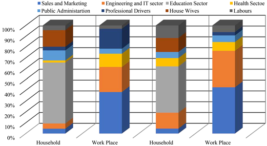
A questionnaire was developed mainly consisting of standardized questions distributed to 1169 participants interviewed in households and working places. In addition to the resident neighborhood type, the factors identified by the participant include gender, age, profession, and car ownership level. As can be seen from Table 2, males outnumber females in both neighborhoods, reflecting their general traffic presentation. The HDR participants seem younger, with over 50% under 25. The working age group for university graduates in the LDR is 58%

Table 1. The characteristics of the study area.

Figure 2. Street infrastructure conditions in the study area (a) HDR street and intersection; (b) LDR street and intersection; (c) HDR public transport facilities; (d) LDR public transport’s facilities; (e) HDR pedestrian facilities; (f) LDR pedestrian facilities.

compared to just 44% in the HDR, which may explain, in addition to the differences in income levels between the two neighborhoods, why the LDR group (42.9%) owns more cars than the HDR group (21.7%). In the household interviews, more subjects work for the HDR than for the LDR, according to the interviewee’s place; more subjects work for the HDR than for the LDR. Professional subjects are twice as common in LDR workplace interviews as in HDR workplace interviews. The HDR group (37.4%) has twice as many business owners as the LDR group (17.3%). The distribution professions in the two neighborhoods differ by the interviewee place; more subjects are working the HDR in the household interviews than in the LDR group. The professional subject in the workplace interviews of the LDR is twice that of the HDR. On the other hand, the business owners in the HDR (37.4%) are twice that of the LDR group (17.3%).

Table 2. Sample size and distribution by area population density group, gender, age, car ownership level.

3.3. The Questionnaire

Open-ended questions were included to seek further explanations for the responses or to put forward suggestions. The questionnaire was distributed to two groups representing the two regions of varying population density, and the questionnaire was distributed to households and in working places. The participants were requested to fill in their answers and return them to the survey’s administrator once completed.

In the first part of the survey, the subject is asked about their socioeconomic characteristics (age, gender, profession, vehicle ownership) and general travel behavior pattern (number of journeys, travel time, and mode of transportation used). The subjects were asked to provide reflections on the mode of transport by assessing the development of infrastructure and operational conditions of the transport mode they use and reflecting on the features of other modes of transportation they do not often use. The responses to this part will describe the infrastructure development index (IDI), a subjective index showing how the subject perceives the municipality’s interest in providing the service to its citizens for that specific mode of transport using a ten-point Likert scale.

The subjects were also asked to rate the perceived safety of the transport mode they use on a ten-point scale, which will define the infrastructure safety index (ISI). A group of questions was introduced to measure an index describing the transport mode attributes, the infrastructure Attribute Index (IAI), which may reflect objectivity in their responses. The modes’ features included in the questionnaire are listed in Table 3.

The pedestrian and public transportation facilities are part of assessing the street infrastructure serving private transport because those facilities are integral to the service and would influence the driving pattern and driver behavior. The list of attributes was short as possible but informative enough to address the main attributes of the service mode, thus encouraging more subjects to participate in the survey. The selection of the attributes is aimed at evaluating the main features that investigated the mode of transport intended to provide for its users. For example, streets should provide for public transport, pedestrians, parking, roadside features, and control devices; therefore, these attributes were assessed. In addition, the selected walking and public transport infrastructure attributes confirm well with the approach used in the evaluation in the reviewed literature [17] [33] .

3.4. Analysis Approach

More than one statistical tool was used in this research, starting with the reliability test—Cronbach’s Alpha—used to assess the stability of the respondent answers to the questionnaire questions. The test was applied to the subject’s responses when rating the mode’s infrastructure development and service attributes. As a rule of thumb, the responses a five-range scale is used: α > 0.9: Excellent; α > 0.8: Good; α > 0.7: Acceptable; α > 0.6: Questionable; α > 0.5: Poor; and α < 0.5: Unacceptable and usually if Cronbach’s alpha of 0.7 and more are deemed acceptable level of reliability [61] . The following sections describe the techniques and tools used in this research in detail.

3.4.1. Descriptive Analyses

This group of tests includes frequency tests, central tendency, dispersion measures for scale data, and contingency table analysis. These tests were applied to

Table 3. Transport mode service attributes.

describe the subject’s rating of transport mode transport attributes and the indices (IDI, ISI, and IAI). The contingency table analysis was used to test the modal share split due to region type.

3.4.2. Data Reduction

The Principal Component Analysis (PCA) was used in EFA to reduce the number of variables describing the service attributes. Even though the number of variables tested for each mode of transport is limited, the tool was still applied, and the developed factors were examined and tested further. The Eigenvalues of the factors must be greater than one and explain at least 70% of the variance to be retained.

3.4.3. Inferential Statistics

Statistical tools were used, including t-test, ANOVA, z-test and one-way repeated measures, and Pearson correlation coefficient (PCC). The t-test was applied to test transport modes’ attribute ratings and indices due to area type. The one-way repeated-measures ANOVA was used to test the agreement between the responses on rating the infrastructure of transport modes development. The z-test was used to test the difference in the modal split proportions, while the PCC was used to test the associations between the proposed indices and the modal share. The significance level used for t-test, chi-square, ANOVA, and one-way repeated Measures (Wilk’s Lambda) is 5%. These tests were applied to the original raw data of the service infrastructure attribute and their factor scores. The correlation between the IDI and ISI with IAI is based on the arithmetic average of the variables that contributed to the reduced and reduced factors for each mode of transport.

3.4.4. Structural Equation Model

A structural equation model (SEM) consists of a measurement and structural models. Measurement models relate observed responses or variables (x₁, x₂, x₃, …, x_i) to latent variables (ξ and η) and sometimes to observed covariates. SEM aims to model the relations between measured and latent variables or between multiple latent variables. The latent variables (constructs) cannot be measured directly but can be inferred indirectly from the observed variables. Models based on structured equations are used primarily to confirm and test hypotheses rather than for exploration. Structured Equation Models help understand different concepts that influence latent phenomena, but they are not always accurate in predicting them. This method estimates coefficients based on hypothesized relationships between variables and cannot find associations other than those specified. Structural equation models can test multiple hypotheses, evaluate them, and analyze their differences to develop a better model (Figure 3). Muthén [62] specifies the full structural model (FSM) for latent variables; η_j as

${\eta }_j=\alpha +B{\eta }_j+\Gamma {\xi }_j+\zeta$ (1)

Figure 3. Path diagram for full structural equation model.

where, j index units or subjects, α: A vector of intercept; B: a matrix of structural parameters depicting the relationships between the latent variables; Γ: a regression parameter matrix for regressing latent variables against observed explanatory variables ξ, and ζ: a vector of disturbances (assuming multivariate normal with zero means).

In the path diagram, exogenous latent measurement models are the x-side variables, while endogenous latent measurement models (CFA) are the y-side variables.

$x_j={\tau }_x+{\Lambda }_x{\xi }_j+{ϵ}_j$ (2)

$y_j={\tau }_y+{\Lambda }_y{\eta }_j+{\delta }_j$ (3)

${\tau }_x$ : the vector of q intercept terms for x-side indicators; ${\tau }_y$ : vector of p intercept terms for y-side indicators; x: vectors of observed exogenous variables; ξ vector of exogenous latent variables; δ: vectors of errors; Λ_x the matrix of coefficients that relates x to ξ. Y is a vector of observed variables referred to as endogenous, η: is a vector of latent variables also endogenous; ε is the vector of errors for the endogenous variables, and Λ_y the matrix of coefficients relating y to η. In addition, the aggregate measure of the residuals is ${\theta }_{ϵ}$ variance or covariance of residuals for x-side indicators ${\theta }_{\gamma }$ variance or covariance of residuals for y-side indicators. SEM evaluations are based on the fit indices for each path coefficient (p-values and standard errors). The overall model fit can be evaluated using good-fit indices that appear flexible in their selection. As a rule of thumb, the factor loading must exceed 0.7 for the factor to account for 50% of the variable’s variance. Still, the literature debate that the threshold may differ by sample size and item frequency distributions, Comrey and Lee [63] suggest cut-offs going from 0.32 (poor), 0.45 (fair), 0.55 (good), 0.63 (very good), or 0.71 (excellent). For this study, a cut-off of 0.5 was considered. The usability of model fitting indices seems flexible. The literature recommends combining at least two fit indices [64] with recommended cut-off values for some indices, as shown in Table 4. Composite reliability measures how much each indicator’s variance is explained by its construct, like Cronbach’s alpha.

$CR=\frac{{\left({\displaystyle \sum {\lambda }_i}\right)}^2}{{\left({\displaystyle \sum {\lambda }_i}\right)}^2+{ϵ}_i}$ (4)

where λ (lambda) is the standardized factor loading for item i and $ϵ$ is the respective error variance for the item i. The error variance ( ${ϵ}_i$ ) is estimated according to the following formula

${ϵ}_i=1-{\lambda }_i^2$ (5)

According to Fornell and Larcker [65] criterion, the average variance extracted (AVE) is a measure of the amount of variance captured by a construct in relation to the amount of variance due to measurement errors.

Table 4. SEM goodness of fit indicators and the related cut-off thresholds.

$AVE=\frac{{\displaystyle {\sum }_{i=1}^n{\lambda }_i^2}}{n}$ (6)

where, λ as above and n is the number of items explained by the construct.

3.4.5. Multinomial Logistic Regression

The multinomial logistic regression is used when the dependent variable is nominal (equivalently categorical, such as private car, walking, and public transportation in this research). This model predicts possible outcomes based on independent variables (scale data, another categorical variable, etc.). If there are n independent observations with p-explanatory variables, and the qualitative response variable has k categories, to construct the logits in the multinomial case, one of the categories must be considered the base level, and all the logits are constructed relative to it. Any category can be taken as the base level; assume category k as the base level. Since there is no order, it is apparent that any category may be labeled k. Let π_j denote the multinomial probability of an observation falling in the j^th category. To find the relationship between this probability and the p explanatory variables, $x_{\text{1}},x_{\text{2}},\cdots ,x_p$ , the multiple logistic regression model is,

$\log \lfloor \frac{{\pi }_j\left(x_i\right)}{{\pi }_k\left(x_i\right)}\rfloor ={\alpha }_{0i}+{\beta }_{1j}{x}_{1i}+{\beta }_{2j}{x}_{2i}+\cdots +{\beta }_{pj}{x}_{pi}$ (7)

where $j=1,2,\cdots ,k-1$ , $i=1,2,\cdots ,n$ . Since all the π’s add to unity, this reduces to

$\log \left({\pi }_j\left(x_i\right)\right)=\frac{\exp \left(\alpha +{\beta }_1{x}_1+{\beta }_2{x}_2+\cdots +{\beta }_k{x}_k\right)}{1+{\displaystyle {\sum }_{j=1}^{k-1}\exp }\left(\alpha +{\beta }_1{x}_1+{\beta }_2{x}_2+\cdots +{\beta }_k{x}_k\right)}$ (8)

For $j=1,2,\cdots ,k-1$ , the model parameters are estimated by the method of maximum likelihood [77] . Practically, statistical software SPSS was used to do this fitting,

Goodness-of-fit Measures

Goodness-of-fit tests such as the likelihood ratio tests are available as indicators of model goodness of fit, as is the Wald statistic to test the significance of individual independent variables [78] . The likelihood ratio test is based on deviance [−2 Log Likelihood (LL)], the significance of the difference between (−2LL) for a selected model minus the likelihood ratio for a reduced model (intercept only). The difference (the chi-square model) is tested without considering interactions in the likelihood ratio model. A chi-square test at a significance level of 5% was performed on the model. Unless the p-value for the model is less than 0.05, indicating an association between explanatory variables and response variables, the null hypothesis will be rejected, stating that no difference was observed between the model with explanatory variables and the model without explanatory variables.

4. Results

4.1. Modal Split

The response rate was 78%, and not all the questions were answered. The modal split in HDR was equally divided by mode of transport, whereas it was shifted towards private passenger cars (57%) and fewer walks (15.1%) in the LDR. The χ² test showed a significant difference in the modal split proportion due to the subject’s region (χ² = 69.8, p = 0.0). The difference between the two regions was pronounced and significant for the passenger car (|z| = 7.1676, p = 0.00) and walking (pedestrians) and (|z| = 7.5105, p = 0.00) but not for public transport (|z| = 0.2495, p = 0.803). In conclusion, we can conclude that there is a shift from the use of passenger cars in the LDR to walking since the modal share of PT remains the same in both regions (Figure 4). While around 46% of the subjects of the HDR have no other choice when they walk to their destination, less than 38% of the subjects in the LDR have no choice but to walk as a mobility mode. The two proportions have no significant difference z = 1.292, p = 0.197).

4.2. Rating Consistency

The reliability test showed consistent responses from the HDR subjects when rating the PT facilities as one component for the street that is mainly designed for private cars in the study area (Cronbach’s alpha > 0.9), which was not the case for the answers for other service attributes that were inconsistent (Cronbach’s alpha < 0.5). The responses of LDR showed varying ratings for calming traffic measures and traffic control devices, like the reactions of HDR. Still, they have relatively better consistency when rating the pedestrian facilities (Cronbach’s alpha = 0.523 for LDR compared to 0.238 for HDR). To some extent, the LDR subjects rated the different features of the PT similarly, but not the subjects of HDR. Overall, the street infrastructure attribute index (IAI) was not placed again across the attributes in both regions; the consistency is still higher. On the other hand, the character in the ratings, the IDI by the private car users, and their perception of the pedestrian and PT facilities were a bit higher for the HDR group (Cronbach’s alpha = 0.644 for HDR compared to 0.284 for LDR); implying that the subjects view the development across the modes of transport similarly, which was not the case for the LDR subjects (Table 5). There was high consistency in the responses related to pedestrian infrastructure, particularly for the crosswalk assessment and, to a less extent, the sidewalk attribute rating

Figure 4. Choice of transport modalities based on respondents’ residential area.

Table 5. The infrastructure attribute and development indices consistency by population density group Cronbach’s alpha (α) by the stated mode of transport in use.

(Cronbach’s alpha > 0.7), indicating high agreement in the ratings and across the regions. The IDI ratings for other modes of transport by the subjects who walk for mobility show an acceptable level of consistency in the HDR (Cronbach’s alpha = −0.754). In contrast, the consistency of the LDR responses is rather unacceptable, indicating different ratings across the three modes of transport.

A different perspective was evident when assessing the public transport facilities rating, which showed no consistency in their rating of the service availability attributes (Cronbach’s alpha (α) < 0.5). HDRs consistently perceive comfort, convenience, and satisfaction, whereas LDRs have a poor perception. Overall, the responses of the HDR group are more consistent than the LDR and approach the level where it could consider acceptable (0.693 < 0.7). In contrast, the value of Cronbach’s alpha of the LDR is 0.342, which is unacceptable, showing an inconsistent service attributes rating. The IDI ratings for other modes of transport by the subjects who use public transportation in their mobility show an acceptable level of consistency in the HDR (Cronbach’s alpha = 0.733) and adequate consistency for the LDR group, which contrasts with the IDI pedestrian infrastructure that was unacceptable.

4.3. Infrastructure Attributes’ Assessment

4.3.1. Rating Assessment

According to the assessment of street infrastructure based on six attributes, parking facilities, street lighting, and traffic calming measures received higher ratings than public transport and pedestrian facilities. The rating of the traffic control devices was the lowest among all other attributes. It appears that LDR subjects rated it higher than HDR except for the lighting attribute, where HDR subjects rated it higher. However, there were no statistically significant differences between the two groups. Streets were rated above mid-scale (5.4). The variance related to street facilities (PT, pedestrian, and parking) is higher than other attributes. Generally, the responses in LDR have higher variation than HDR, except for the lighting attributes assessment. Table 6 shows that the subjects, irrespective of their neighborhood, recognized poor standards and conditions of the crosswalks and rated them on the lower part of the scale with no statistical differences due to their residence place. Despite the ratings of the sidewalk standards and operating conditions being higher than the crosswalks’ ratings, they are still less than the mid-point scale, with no statistical difference between the two groups’ answers. However, the subjects in both groups rated the infrastructure as encouraging to comply with traffic rules, and it was above the mid-point of the scale, a bit higher for the HDR group. The subjects may state their behaviors rather than the infrastructure in their responses.

Table 6. Infrastructure attributes descriptive statistics by mode of transport and neighborhood type.

Both groups’ participants rated the waiting time and area poorly; the HDR’s average rating is slightly higher (3.99 compared to 3.38 for the LDR); the difference is marginally statistically insignificant. Because they are related, stops and terminal facilities are rated similarly to waiting time attributes, and their ratings are statistically insignificant. HDR rated spatial coverage highest (6.62), statistically different from LDR (5.29). Both groups rated temporal availability above the mid-point scale without statistically significant differences. Like other attributes, the HDR group rated customer satisfaction higher than the LDR group. There is a significant difference between the customer satisfaction ratings of the two groups. Regarding comfort and convenience, both groups placed almost around the scale’s midpoint with no statistical differences (Table 6).

4.3.2. Factor Analysis and Data Reduction

The difference in ratings indicates that assuming equal weights for the service attributes to calculate the IAI may not be the appropriate measure. The principal component analysis was applied to reduce the number of variables and define variables contributing to an established factor describing a particular dimension of the facility (Table 7). Two factors can explain the variation in the data relating to street infrastructure in the two neighborhoods explaining the original data

Table 7. Infrastructure attributes factors by mode of transport: principal component analysis.

of 60.5% and 70.4% for the HDR and LDR, respectively. The HDR data’s two factors are facilities (Public transport, pedestrian, and parking), traffic management, and control factors (Control devices, calming measures, and lighting). The facilities factor was positively correlated to PT facilities and, to less extent, pedestrian facilities and negatively correlated with parking facilities. The traffic control devices attribute was associated positively with the calming measure attribute’s second factor. Still, the lighting attribute is negatively related to the second factor, weak though. Different factors’ structure is observed in the LDR data. The first factor explains 47% of the original data variation. According to the association order, it positively correlates to calming traffic measures, control devices, and pedestrian and PT facilities. The second factor that describes around 24% of the original data variation is positively correlated to the lighting attribute and negatively related to the parking attribute, like the association in the HDR first factor, implying that parking standards and activities reduce the infrastructure rating in both regions.

Based on these two factors, both datasets explain 74.25% and 72.82% of the original variation in the HDR and LDR, respectively (Table 7). The crosswalk attributes’ components and degree of association with the composite factors are similar for both datasets, with a positive correlation exceeding 0.88. The sidewalk paving surface and height reflecting the convenient pedestrian experience when walking in the HDR have a higher correlation with the sidewalk factor than the sidewalk width, which is also positively correlated; the little correlation is due to the facility encouraging compliance with rules. In contrast, the correlation with sidewalk factors was higher for the sidewalk width than the surface material or the height in the LDR environment. Even though the correlation with facility encouraging compliance with rules attributes is higher than HDR (0.652).

Two factors can explain 64.43% and 55.93% of the variation in the original data, one for each data group assessing the public transport infrastructure, which is less than the defined thresholds in this study (70%). However, about 50 to 60 percent of explained variance can be accepted in social science Hair et al. (2010). The first factor of the HDR mainly includes all the attributes except the waiting time attributes, explaining 47.85% of the variation of original data. The second factor, representing the waiting time and area attribute, accounts for one-sixth of the original data variation. All attributes positively correlated with the established two factors. Comfort and convenience correlate with the first factor (0.83), while temporal availability has the lowest correlation (0.638). Spatial and temporal availability attributes positively correlate with the 1st factor of the LDR, while waiting time is negatively correlated. The comfort and convenience factor describe the remaining three characteristics with a positive correlation; the highest correlation is with customer satisfaction (0.811), and the lowest is with terminal facilities (0.67), indicating a small range and similar association (Table 7).

4.4. Infrastructure Development Index

4.4.1. Rating Consistency

The hypothesis that the subjects’ assessments of the infrastructure for private cars, pedestrians, and public transportation are unaffected by their commuting mode of transportation was tested using a one-way repeated measures analysis of variance. At a significant level of 5%, the modes of transport attributes were rated differently by the subjects in the two groups. In Table 8, participants who travel by car assess the three modes of transport infrastructure development significantly (Significance of F-Test, Table 8). In contrast, subjects walking for mobility in the HDR group rated the infrastructure of different modes of transportation similarly, which is not the case for corresponding participants in the LDR group; the test result was insignificant, suggesting a similar appraisal of transportation infrastructure development.

4.4.2. Rating Assessment

The HDR subjects who used private passenger cars rated the street (2.99) lower than their IDI ratings for pedestrian facilities (4.59) and public transportation infrastructure (5.05). On the other hand, LDR subjects rated street IDI (4.75) higher than pedestrian infrastructure (3.88), but lower than public transport (5.12); however, the LDR group rated street IDI higher than HDR (t = −7.78, p = 0.0). Those who used a private car rated public transportation infrastructure similarly but pedestrian infrastructure differently (Table 9). In both groups, walkers rated pedestrian IDI higher than street IDI and public transportation IDI. For the three modes of transportation for LDR groups, the assessment lies within a narrow range (4.07 to 4.39), supporting the previous F-test result in Table 8. HDR walking groups rate public transport facilities higher than pedestrian facilities, but street IDI is underrated. Passenger car infrastructure was significantly rated differently between the two groups (t = −0.835, p = 0.00),

Table 8. Infrastructure mode rating across different facilities by the mode of transport in use and the test group: Reparted measurement analysis of variance analysis.

Hypothesis degree of freedom 2 error degree of freedom.

Table 9. Infrastructure development assessment by mode of transport and test group.

whereas the other two modes of transportation were not significantly different. In the LDR, public transport users rated the level of development for the three modes of transportation similarly, which is not the case in the HDR group, where public transport is almost double that of the LDR and slightly above pedestrian IDIs. On average, it is 1.71 points higher than their passenger car rating. All modes of assessment showed significant differences between the two groups.

On average, pedestrian infrastructure received the lowest assessment, followed by the street, while public transport rated higher (4.6) and closer to the mid of the scale. In fact, with two exceptions related to the public transport commuter in the HDR group who rated the pedestrian (6.22) and public transport (6.62) facilities as being above the scale, all other assessments below (5). Figure 5 suggests the private car commuter in the HDR underrate the street IDI while the public transport commuters in this group rated the facilities higher than pedestrians or street IDI.

4.5. Infrastructure Safety Index

4.5.1. Rating Assessment

The safety index for each mode of transport value is placed at the scale’s mid-point or below. Except for the pedestrian index, the LDR indices are higher than the HDR. The public transportation and pedestrian indices mirror each other but in the opposite direction. Pedestrian facilities ISI of the HDR (5.03) was rated higher than the LDR (4.61), while the public transportation facilities of the LDR (5.06) were rated higher than HDR (4.62). The street ISI of the LDR (4.71) is marginally higher than the HDR (4.6). There was no significant difference between the ISIs due to the group of respondents for any mode of transport.

4.5.2. Safety and Association with Infrastructure Perception

The IAI’s factored and unfactored indices for each mode of transport were used to test the association between perceived safety levels and perceptions of transport infrastructure facilities. The correlation analysis for the un-factored data covers the individual attributes tested. The IDI of the three modes of transportation infrastructures was also correlated with the safety indices. There were no

Figure 5. Transport facilities’ IDI by mode of transport and population density group.

statistically significant correlations between the two-neighbourhood street IAI factors and the perceived safety index, except for the first factor of the LDR. A positive correlation exists between safety perception, public transportation facilities, traffic control devices, and calming measures, but it is insignificant. At the same time, there is a negative correlation between safety, lighting, and parking attributes. Despite their weak and insignificant significance, HDR groups have slightly higher correlations (Table 10). Furthermore, there was no significant correlation between IDI and perceived safety (ISI).

Based on the factored data, the reduced variables (factored data) of those who walk for commuting show statistically significant positive correlations, but not as high as their corresponding variables for the LDR and higher than the factored data. None of the tested correlations for the factored or unfactored data of the LDR was statistically significant. For HDR, perceived pedestrian safety and perceived pedestrian IDI are positively correlated (r = 0.445, p = 0.00) but inferior and statistically insignificant for LDR (r = 0.252, p = 0.084). In Table 10, the correlation between pedestrian ISI and IDI is positive and significant for the HDR group but insignificant for the LDR group. The association between the subjects’ perceived public transport infrastructure safety level shows statistically significant positive correlations for the HDR data set, indicating poor significant correlation and even very poor and insignificant for the second factor describing comfort and convenience.

There is no distinct trend in Table 10 explaining the difference in the association due to the method employed in establishing the attributes’ indicator. The correlation between safety and the 1st established factors for HDR data is more robust than that with average availability, representing the arithmetic average of the variables contributing to the 1st established factor. By comparison, the second factor, the service comfort perceived by the LDR, has a relatively small impact based on the simple arithmetic average. In Table 10, the correlation

Table 10. The association between perceived safety with transport infrastructure attributes/factored indices, and the IDI by the commuting mode of transport.

**. Correlation is significant at the 0.01 level (2-tailed).

between ISI and IAI factored or unfactored is somewhat higher than other correlations reported between pedestrians and street infrastructure. Overall attributes averages correlate better with safety for both data sets (r = 0.326, p = 0.0, against r = 0.262, p = 0.0 for HDR, and r = 0.485, p = < 0.001 against r = 0.313, p = 0.002 for LDR group). As with the pedestrian infrastructure association trend, the public transport ISI positively correlates with IDI for the HDR group (r = 0.285 p = 0.001) but negatively insignificantly for the LDR group (r = −0.123, p = 0.231).

4.6. Interrelation Analysis

4.6.1. Indices Descriptive Comparison

This section aims to examine the interrelationship between the aggregated three indices for the two groups. In Figure 6, all attributes for each mode of transportation were averaged, regardless of the mode of transport used for commuting. The street IAI of the HDR for passenger car traffic (4.85) is the lowest compared to the other two modes of transport and to its corresponding LDR (5.34); the difference was insignificant, with only 0.49 points difference. IAI of pedestrian facilities in HDR and LDR differ statistically significantly (5.00 and 3.87, respectively). HDR (5.00) is at the scale’s midpoint, higher than LDR (3.87) by (1.13). Among the other indices and groups of participants, the HDR group’s IAI for public transportation (5.36) was statistically different from that of the LDR (4.75) by 0.614 points. Among other modes, the HRD group’s street IDI assessment was the lowest (3.358), statistically different from the LDR group’s (4.058). Public transport facilities had the highest IDI, with 5.487 for HDR, the only index above the midpoint, and 1.351 points greater than LDR (4.136). For pedestrian IAI, the HDR index (5.02) is significantly higher than the LDR index (3.875), with a statistically significant difference of 1.14 points. A single ISI was used to rate each mode of transportation, with HDR’s group rating being 4.6, while LDR’s group rating was 4.71, a difference of 0.11 points between the two. The ISI difference for public transport facilities is the largest (0.44 points; 4.62 and 5.06 for HDR and LDR, respectively), almost equal to that of pedestrian facilities (5.03 and 4.61 for HDR and LDR groups, respectively). On average, the subjects in both groups perceived the three modes’ infrastructure attributes indices (4.96) more than the safety index (4.77) or the overall level of development index (4.32). The average IAI for the three modes of transport for the HDR exceeds that of the LDR group by 0.42 (5.07 and 4.65 for HDR and LDR groups, respectively). The IDI difference is higher (0.60), but the overall average is lower (4.62 and 4.02 for HDR and LDR groups, respectively). As assessed in the HDR group, the ISI for the three modes was 4.75, while the ISI for the LDR group was 4.79, which looked almost identical by only 0.04 points difference. Overall, public transportation infrastructure (IAI, IDI, and ISI) was appraised the highest (4.9), while pedestrian infrastructure was the lowest (4.57), which was marginally different from street environments (4.49).

Figure 6. Infrastructure assessment indices by mode of transport and population density group.

In terms of indices, the IAI for private car traffic was the highest (5.10), while the pedestrian infrastructure was the lowest (4.44), leaving the IAI for public transportation close to that of street traffic (5.05). Compared to the street and pedestrian infrastructure, public transportation infrastructure scored 4.81 in the IDI, 1.1 points higher. Among the three modes of transportation, the ISI in public transport (4.84) was slightly higher than in pedestrian infrastructure (4.82). In comparison, the ISI in street infrastructure (4.65) was marginally lower than in public transportation. LDR generally rated street infrastructure better than HDR, which then rated pedestrian and public transportation facilities better than LDR.

4.6.2. Indices Interrelation Analysis

The interrelation analysis of these indices showed a positive trend (Figure 7), but no association can be statistically significant between the IAI and ISI (r = 0.13, p = 0.37) or with IDI (r = 0.063, p = 0.66). However, the ratings of the facility IDI are positively related to the perceived safety assessment, low correlation though (r = 0.31, p = 001). The LDR participants rated the street infrastructure (5.44) higher than their ratings of the facility ISI (4.7) and IDI (4.1), which is also like the HDR group rating trend. The IAI and ISI ratings are poorly correlated (r = 0.045, p = 0.73). At the same time, the IAI is weakly negatively correlated with IDI rating (r = −0.23, p = 0.22), implying that subjects rated the street attribute infrastructure high while they perceived its development as low, which

Figure 7. The relationship between the three different infrastructure indices.

in turn, was not proven to be related to their assessment of the ISI (r = 0.05, p = 0.728). The HDR group rated the pedestrians’ facilities’ indices around the scale’s mid-point. Figure 7 indicates a moderately significant correlation between the three indices, with the highest being between the IAI and ISI r = 0.51, p = 0.00), and the lowest is between IDI and ISI (r = 0.42, p = 0.00), which does not differ from the relationship between the IAI and IDI (r = 0.45, p = 0.00). The LDR group rated pedestrian facilities’ IAI and IDI similarly (3.9), lower than the ISI rating. Apart from the relation between the IDI and ISI, which was marginally significant (r = 0.32, p = 0.025), the association between other indices was very low and insignificant (p > 0.025), with a coefficient of 0.11 for IAI-ISI and 0.032 for IAI-IDI relationships.

The HDR group rated public transportation facilities’ IAI and IDI above the mid-point of the scale with a minor difference of 0.13 points with a moderate correlation (r = 0.56, p = 0.00), the highest reported among all other indices. The ISI was rated as 4.62 and was significantly low correlated with IAI (r = 0.33, p = 0.00) and IDI (r = 0.29, p = 0.00).

The ISI rating of the LDR (5.06) was the highest compared to IDI (4.14) and the IAI (4.75), which were positively and significantly correlated (r = 0.48, p = 0.00) but not with IDI that showed negative insignificant very low correlation (r = −0.06, p = 0.67). The two later indices were positively moderately correlated (r = 0.47, p = 0.008).

4.7. Structural Equation Modelling (SEM)

The structural equation model combines confirmatory factor analysis (CFA) and regression analysis. This study covers two perspectives, the measurement model and the structural Model (Figure 8). The measurement model correlates the latent variables and their indicators, while the structural model models relationships between unmeasurable factors. The first Model aimed at developing the latent variables describing the infrastructure attributes of the three investigated modes of transport (Private car “street”, walking “pedestrian”, and public transport). The CFA revealed three latent variables describing the infrastructure attributes for streets, pedestrian, and public transport loading factor for all attributes rated by the subjects was not always greater than 0.5, the minimum acceptable threshold for indicators inclusion in SEM models according to the literature; however, if the overall model goodness of fit measures were adequate, some indicators can still be retained in the Model if their values were below this threshold. Other models included variables describing socioeconomic characteristics (Resident area, gender, and car ownership) and modal choice. The modal choice and car ownership variables are binary (e.g., if the respondent uses public transportation frequently, the modal choice for the bus will be one, and if they walk or drive, it will be zero).

4.7.1. Confirmatory Factor Analysis

Confirmatory Factor Analysis (CFA) was computed using AMOS to test the

(a)(b)

Figure 8. CFA and FSM variables and coefficients (a) CFA; (b) FSM.

measurement models; factor loadings were assessed for each item for each Model. The factor loadings for the infrastructure attributes-based Model are significant (p < 0.05) with estimated standardized coefficients exceeding 0.5 except the traffic control item (λ = 0.436), and it was kept in the Model because the Model’s goodness of fit indicator satisfies the requirements of sound models. When car ownership and public transportation are included in the Model, the estimated path coefficients are significantly lower than 0.5. However, the coefficient for public transportation modal choice is insignificant if only included. The model-fit measures were used to assess the infrastructure attribute-based model’s overall goodness of fit (CMIN/df, CFI, TLI, IFI, and RMSEA). The subjective infrastructure assessment IDI was added, producing a significant correlation with a standardized coefficient of (0.525). Including the pedestrian or streets, IDI failed to have a significant correlation with their latent variables, including the pedestrian or street. All values were within common acceptance levels, and the NFI was approaching the 0.9 cut-off value. To test the consistency of latent construct measures (factors), the CR and the AVE were tested. Composite reliability reached the limit of 0.70 (from 0.782 to 0.875), and AVE values exceeded 0.50 for Street IAI (λ = 0.563) and Pedestrian IAI (λ = 0.65) but not the Public Transport IAI (λ = 0.423).

IAI street measures include traffic control (λ = 0.436), traffic-calming measures (0.698), pedestrian facilities (0.918), and public transport facilities (λ = 0.863). Other items or observed variables (lighting and parking) were insignificant and with very low path coefficients. The observed variable that is proven significant in describing the pedestrian IAI were sidewalk sufficiency (λ = 0.457), crosswalk safety (λ = 0.890), visibility (λ = 0.857), and sufficiency (λ = 0.928). Sidewalk width, curb height, and conditions were insignificant; therefore, were not included in the Model.

For public transport IAI, three out of the observed six attributes were found to have a significant path coefficient with an estimate exceeding 0.5, namely service convenience (λ = 0.731), comfort (λ = 0.772), and coverage (λ = 0.51). The model-fit measures for other measurement models that include car ownership and public transport as a modal choice as indicators for the latent variable of public transport IAI showed acceptable values for the two models (the inclusion of car ownership only; the use of public transport variable only) indicate that Chi-square divided by Degree of Freedom, RMSEA, and IFI and CFI are within acceptable cut-off values (≥0.90). The TLI approaches 0.9, telling a good fit with the data. For the model including both variables, CMIN/df and RMSEA are within acceptable limits, and only the CFI and IFI values are close to 0.9, but not the TLI and NFI; According to the literature, two indicators were within the acceptable cut-off model, suggesting that this model is barely acceptable as a model for developing public transport IAI latent variables. For those three models, the composite reliability is more than 0.7, while the AVE, like the infrastructure attributes-based model, is less than 0.5 (Table 11).

Table 11. SEM analysis: Model goodness of fit indicators.

4.7.2. Full Structural Model (FSM)

Several hypotheses were tested to examine the relationships between the three developed latent variables. It is possible to elaborate on the relationships by describing how street and pedestrian IAIs impact public transportation IAI. Models describing other relationships were not sound enough and were statistically insignificant. This part of the study assessed the impact of street and pedestrian IAI on public transport IAI. First, the infrastructure attributes-based models showed that the impact of the pedestrian IAI latent variable was positive and significant on public transport IAI (b = 0.296, t = 2.919, p = 0.004 < 0.05), supporting the alternative hypothesis stating that there is an impact of pedestrian IAI on public transport IAI. The impact of street IAI was also positive but insignificant (b = 0.063, t = 0.503, p = 0.615 > 0.05), supporting the null hypothesis stating there is no impact of street IAI on public transport IAI. The model fit indices and hypotheses results are presented in Table 12 and Table 13. The remaining models are based while still testing the same hypothesis; the IDI indicator was excluded from basing the analysis on the infrastructure attributes and the modal choice of bus and car ownership to study the impact of the region where the respondents reside and the gender on the tested relationship. Table 13 shows that including bus as a modal choice and car ownership variables provides similar results to attribute-based models.

Table 12. SEM analysis CFA coefficients and their significance.

Table 13. SEM analysis FSM coefficients and their significance.

A further analysis divides the data into groups based on residence area (HDR and LDR) and gender (male and female). In this model, street IAI is not significantly associated with public transport IAI; pedestrian IAI is significantly associated with the latter; the same holds for the male group model. These four models’ measures of the overall goodness of fit did not meet the acceptable cut-off values except for those related to CMIN/df and RMSEA; on the female group models, RMSEA (0.087) was out of tolerance (<0.08). The latent CR and AVE in the last model of the female group are below acceptable levels; their corresponding values in the HDR and LDR, and the male group, are within acceptable levels.

Data fit poor based on these models’ goodness of fit measures. The paired comparison between the models divided by area of subject’s residency revealed a significant difference between the estimates of people living in HDR or LDR (cmin = 7.23, p = 0.0007). The estimates of males and females are not significantly different (cmin = 0.727, p = 0.122).

4.8. Modal Share and Infrastructure Perception

4.8.1. Modal Choice Discrete Models

Multinomial Logistics regression (MLR) for the modal choice results is summarized in Table 14. Utility function equations were developed to explore the modal choice of road users between private passenger cars, walking, and public transport, as well as the contributing variables and factors. The IAI, IDI, and ISI were examined along with trip and road users’ socioeconomic characteristics; none of the infrastructure indices significantly influenced modal choice. The respondent’s modal choice was associated with a limited number of variables, including trip and travel time, number of trips, car ownership, and the area where the respondent lived. Ten models were developed based on many tested models, which are potentially valid for one or more aspects of soundness and goodness of fit.

The pseudo R² in MLR is the same as the R² in ordinary least-squares linear regression, which is the proportion of variance explained by the model. It is better if the regression model has a higher value, even if it cannot be easily interpreted; the models will be validated using Nagelkerke, index which was between 0.048 and 0.706 (Table 14). Five models have a value greater than 0.50 and use trip time, total travel time, and trips as predictor variables alone or combined with car ownership level as a contributing factor. Nagelkerke pseudo-R² values for one-variable predictor models are low, but those with more than one predictor have relatively high values. Total time, trips, and car ownership have the highest values for model number 10, which is 0.706.

Partial test

The Likelihood Ratio Test shows the contribution or influence of each independent variable on the transport modal choice. The likelihood ratio test hypothesizes that the variable contributes to the reduction in error measured by the −2-log likelihood statistic suggesting that the regression coefficients in the model

Table 14. Multi logistic regression models: goodness of fit, model significant variable and correct classification.

RM: Reduced Models PC: Private Car PT: Public Transport.

are not equal to zero. If the test’s significance is minor (p-value < 0.05), then the variable significantly explains the mode choice. Among many models, the models summarized in Table 14 were statistically related to the dependent variable. The p-values of all tested variables in the ten models are less than 0.05, indicating that they contribute significantly to explaining the used mode choice. A person’s transportation modal choice is influenced by the amount of time spent traveling, the ownership of a vehicle, the total number of trips, and the trip time (the time spent traveling for a particular purpose).

Model Fitting Test

According to the model fitting test results, the variables added to the model improve the model over the intercept alone (i.e., without variables). H0 indicates that no independent variable influences the dependent variable; HA suggests that at least one independent variable affects the dependent variable significantly. If the calculated chi-square value exceeds the tabulated value at a significance level of 5%, the H0 hypothesis is rejected. The ten models developed all have p values below 0.05, which indicates that the full model can significantly better predict the dependent variable than the intercept-only model.

Model Goodness of Fit test

The goodness of fit test explores if there is a difference between the frequency of observation with the model or the frequency of expectations. The model is considered to fit the data if its p-value is above 0.05. The MLR procedure in SPSS reports Pearson and Deviance goodness-of-fit statistics. According to Table 14, most models with high Pseudo R² that exceed 0.5 have a p-value greater than 0.05 for either Pearson or Deviance or both, indicating that they fit the observed data. The Pseudo R² of models 1, 3, and 7 is small, but their p-values are greater than 0.05, suggesting a good fit.

Classification

This analysis shows how many observations were correctly classified by the models; the range of percentages ranges from 42.9% to 76.3%. There is a higher proportion of correct classification for models with a higher pseudo R² (above 65%) and a lower proportion for models with a pseudo R² of less than 0.5. The percent of correct classification differs by mode of transport; passenger car correct placement was as low as zero percent and as high as 78.4%; the corresponding range for walking as a mode of transportation was 3.2% and 61.7%. Public transportation users are more likely to be classified correctly than other modes of transportation, with a percentage range of 34.4% to 100%. All three modes of transportation are classified correctly similarly in models 9 and 10, which have the highest overall correction classification and highest Pseudo R². The percent of correct classification differs by mode of transport; passenger car correct placement was as low as zero percent and as high as 78.4%; the corresponding range for walking as a mode of transportation was 3.2% and 61.7%. The percentage of correct classification of those who use public transportation is higher than the other modes and ranges between (34.4% and 100%). All three modes of transportation are classified correctly similarly in models 9 and 10, which have the highest overall correction classification and highest Pseudo R².

Model Development: Parameter estimates

Considering the null hypothesis, all regression coefficients in the model should equal zero; the tested model’s small p-value (<0.05) indicates that at least one regression coefficient does not equal zero. The logit functions in Table 15 compare the choice of the reference mode with the remaining modes of transportation. The first group of models uses a passenger car with walking and public transport, while the second group compares walking with public transportation. Instead of walking and driving, the last models’ group used public transportation as a reference mode. A variable parameter coefficient differs according to the reference mode (e.g., the coefficient of total time (0.019) influences the choice of passenger cars in model 1 more than walking); however, it has a lower influence (−0.019) on walking as compared to passenger cars.

The majority of the variables’ coefficients that are related to walking as reference mode are significant (p < 0.05), indicating that they are different from zero, and those with poor significance are related to passenger car attributes (Models 4, 8, through 10). Passenger cars are chosen as the reference mode in models four through seven; one of the three tested variables were included as a predictor; passenger car ownership and area type coefficients are not zero, as indicated by their p values (<0.05). The car ownership coefficient varies from zero for models 9 and 10 when comparing public transport to walking or vice versa. Next, model 10, incorporating total travel time, total trips, and car ownership, will be discussed, which has proved to fit the observation data with high accuracy (75.9%).

Public transport and walking attributes are not significantly different from zero compared to passenger cars, according to Table 15. The multinomial log-odds coefficient for public transport is 0.017 and 0.02 higher than passenger cars and walking, respectively. In terms of the number of trips taken by public transport, the coefficient is 1.065 and 0.818, which is higher than the number of trips taken by passenger cars and on foot. Compared to public transportation and passenger cars, the passenger car factor contribution is insignificant, or it does not contribute at all to walking compared to passenger cars and vice versa; however, it is significant in comparison to public transportation.

Table 15. Multi logistic regression: parameters estimate and their significance.

4.8.2. Infrastructure Incidences and Aggregated Modal Share

A presentation of the association between the modal share and the mode of transport indices showed a slight difference between pedestrian facilities’ IAI and IDI and the modal share.

It offers a positive association between the two indices (IAI and IDI) with the modal share for the LDR group; as the index increases, the modal share increases. The coefficients of determination were 0.93 and 0.27 for IAI and IDI, respectively.

Figure 9 also indicates a marginal difference between the two indices for pedestrian infrastructure, while a wide range exists for private car indices. In contrast,

Figure 9. The relation between infrastructure assessment and modal share.

no evident trend explains the relationship between the modal share of the HDR and its infrastructure attributes. There was no association between the IDI and modal share (r = 0.08). A solid negative association (r = 0.98) between the modal share and IAI decreases as the service attribute increases. The absence of other choices in the HDR leaves the subjects captive to one mode regardless of its attribute, which is not the case in the LDR. The gap between the IAI and IDI for the private car environment is enormous (2 points), while it is minimal for the other two modes of transport and smaller than that of the LDR. As another mobility indicator, the number of trips introduced and tested differs by the responding group, and its relation to the IDI and IAI differs.

Figure 10 also shows the aggregated IDI across the three modes of transport of the HDR (4.66), a statistically significant difference from the LDR (4.0). In contrast, the difference due to the subject group of the IAI was insignificant, with only 0.276 points; the mean of the LDR group is (4.98) compared to (4.7) for the HDR. There was no significant difference between the number of trips of the two groups, although the HDR group reported (5.1) compared to (4.8) trips per day for the LDR. The group’s relationship between trips and the infrastructure indices differs in magnitude and direction (Figure 9). The number of trips of the HDR is positively correlated with the IAI (r = 0.452, p = 0.00) and with IDI (r = 0.475, p = 0.00). In contrast, the correlations were negatively insignificant for the LDR group, with coefficients of −0.148 (p = 0.434) and 0.162 (p = 0.219) for the IDI and IAI, respectively. Irrespective of the group, the association between trips and the indices was significantly positive (r = 0.37, p = 0.00) and r = 0.29 (p = 0.00) for IDI and IAI, respectively). The above association reflects the relation between the two indices, as the correlation was positively significant for the HDR (r = 0.642, p = 0.00) and negatively insignificant for the LDR (r = −0.146, p = 0.44).

Figure 10. The association between number of trips and infrastructure indices.

5. Discussions of Results

This study’s objective was to assess the road users’ perception of the development of different infrastructure modes and their interrelations; and if it is related to the service attribute and embedded safety level or the mode they commonly use. It also investigates how this would influence their modal choice pattern and whether it differs by the assessor’s environmental background. The modal choice models were developed at individual and collective (aggregated) levels. A two-group from two different regions in Amman with varying population densities and infrastructure development were asked to rate the infrastructure of three modes of transportation (Private car, walking, and public transport) from three perspectives: development level, service attributes, and safety. Several attributes were selected describing what the users would expect to receive once they use the mode of transport of interest. Streets that provide for private car traffic and other traffic types (pedestrian and public transportation) are perceived to have similar attributes across the two regions, with some advantages for the LDR, which reflects a lower population density and a more modern neighborhood setup. The main concern, irrespective of the group, was the adequacy of traffic control devices, including marking, signing, and signaling, which was indicated by their low rating of the provided level of safety.

5.1. Road User Perception

Subjects from the two groups evaluated pedestrian infrastructure attributes like the level of infrastructure development in their area of residence, which differed significantly from the other area. Their concern was the crosswalk conditions rather than the sidewalk. With more than 30% of the sample size of the HDR group walking for their destination, they appraised the safety as higher than the LDR with less than 10% walking. The association between the service attributes and the level of development for the HDR group was higher, which may reflect their experience; still, there was a contradiction between how they rated the attributes low and how they valued safety relatively high. The consistency of the three indicators of the LDR group assessment of pedestrian infrastructure seems higher than the HDR. In fact, and overall, the consistency in the appraisal across the modes was an issue that needed further investigation.

The LDR group perceived the safety of public transportation facilities as higher than the other two modes of transport, even though they are concerned about the waiting time and area as it may sometimes involve risk. The HDR group appraised the safety of public transport and private car infrastructure similarly. The level of development of the public transportation facilities was rated as the pedestrian infrastructure (IDI), which is quite understandable, as walking trips complement the public transportation service. 121 Those who use public transport in the HDR group rated its development relatively high, two times the LDR group’s rating. In addition to the concern about the waiting area, the stops and other terminal facilities’ conditions were perceived as low. On the other hand, the two groups acknowledged the availability of the service temporally and spatially despite being a general complaint from the public, which may be due to being captive to the service and knowing how to manage around. Nevertheless, there was a substantial difference in their perception of the overall development of the infrastructure as the LDR group rating was significantly far below the HDRs.

To conclude Therefore, it is possible to falsify the first hypothesis and conclude that the road-users perception of transport infrastructure differs by the region and the characteristics in which the subject resides. Further, there is a difference between their assessment across the modes within each group. The verification of the second hypothesis is not straightforward. It could be stated that the LDR group has a similar perception of the transport infrastructure development irrespective of the mode they commonly use, which is not the case for the HDR group, which has a significant difference in their perception of the other modes of transport.

The conclusion partially confirms some literature showed that the perception of infrastructure is related to its use and safety perception [4] [16] [18] confirm what Azik et al. [7] who reported that drivers’ perceptions and evaluation of the infrastructure differ from one country to another and Manaugh and El-Geneid [22] [23] who suggested difference perception within the same urban setup. For pedestrian and public transportation infrastructure attributes, HDR subjects showed consistent responses compared to LDR. However, LDR responses of streets are significantly higher despite street infrastructure responses’ lower reliability than the other two modes. Among SEM-related attributes, reliability, Cronbach’s alpha (α) was higher, rated 0.83, 0.88, and 0.78, suggesting reliable assessments range from good to excellent for those items incorporated in the unobserved construct, explaining why reliability would be less when all indicators are included (Table 5).

5.2. Infrastructure Perception Indices Models and Interrelation

Using exploratory factor analysis—PCA, two factors were identified for each group; these factors were poorly correlated with safety appraisals, as with the original qualities, irrespective of group. Despite the reduced factors explaining a proportion of the variation in the original data variation that does not exceed 75% on the best (pedestrian IAI), still, their association with other indices is relatively better than the association based on the original variable, indicating the need to consider giving different weights for the variables. Future research can address the issue of weighing road infrastructure attributes from different perspectives. Consequently, both groups perceive the infrastructure attributes index IAI (4.96) better than the safety index (4.77) or overall level of development index (4.32), suggesting that reflecting on service indicators is higher than a general impression, which confirms De Oña et al. [16] findings. The IAI of private car traffic was the highest at the indices level (5.4), and the pedestrian infrastructure was the lowest (4.4).

The subjects’ ratings of the infrastructure IDI for private cars, pedestrians of the LDR, and public transportation are affected by their commuting modes. In contrast, subjects walking for mobility in the HDR group rated the infrastructure of different modes of transportation similarly. The IDI public transportation infrastructure was the highest rated (4.81), a slight difference from the pedestrian rating (4.45) and a deviation of one point from the street environment rating (3.71). The average of the three indices of public transportation infrastructure was the highest (4.9), and pedestrian infrastructure was the lowest (4.57), which was marginally different from the street environment (4.59). The low perception of pedestrian infrastructure is consistent with literature findings [21] [29] [31] [33] . There was minimal difference between the safety conditions among the three modes; safety assessments for the three modes were below the mid-scale (the lowest rating is 4.66 for the street environment, and the highest for public transportation (is 4.84); implying that the safety is impeded in the mindset of the users irrespective of the mode in-use. Safety is closely associated with modal selection and service perception in the literature [21] [34] [35] [41] [43] . The average of the three observed indices has a weak correlation. The association is more robust for HDR responses, which are almost always positively correlated, except for the relationship between street IDI and public transport IDI. Public transport’s IAI-IDI for the HDR was 0.56 compared to 0.47 for the LDR; the street’s IAI-ISI was 0.51 compared to 0.11 for the LDR.

Based on SEM-CFA, pedestrian and public transport facilities and calming traffic measures influence the street IAI’s construct. To a lesser extent, traffic control devices, lighting, and parking conditions contribute insignificantly and minimally. The pedestrian IAI construct is mainly related to crosswalk characteristics and, to a lesser extent, sidewalk characteristics. The comfort and convenience and, to some time, bus stop conditions are better correlated to the public transport IAI construct than the service coverage or the user perception of the development index. Only the public transport IDI contributed to the public transport IAI construct, where none of the pedestrian or street IDI were related to their constructs. In the CFA, fewer variables were incorporated into the constructs than in the EFA. The consistency of the ratings of CFA variables was higher than those of EFA. SEM-FSM showed significant positive impacts of pedestrian IAI on public transport, but insignificant impacts of street IAI. Streets and pedestrian constructs do not significantly contribute to explaining streets; the same is true for pedestrian constructs. While there is a significant difference between the developed models due to the subject’s residency, also contributing to verifying the 1st hypothesis, there is no significant difference due to the subject’s gender. These findings match well with the literature [38] [43] [45] .

To conclude and based on SEM, EFA and descriptive analysis, it seems that transport system users’ perception of transport infrastructure attribute-based is different from their general or overall perception; thus, the 3rd hypothesis could not be verified.

5.3. Infrastructure Perception and Transport Mode Choice

Generally, the observed average indices across all modes of transport are weakly correlated with the number of trips made by the subject (r < 0.5). The correlation is higher for HDR responses (r = 0.48 for IDI and 0.45 for IAI, compared to only −0.15 and −0.16 for LDR). There is a positive relationship between modal share and infrastructure IAI (0.98 for HDRs and 0.96 for LDRs) but a weaker association with IDI (0.52 for LDRs and 0.1 for HDRs), which means the higher the index that describes infrastructure attributes, the higher the modal, whereas this is not the case for their responses general impression (IDI). Regardless of the respondents’ group, there is a significant positive weak significant correlation between trips and aggregated indices (r = 0.37, p = 0.00 for IDI and r = 0.29, p = 0.00 for IAI). Discrete modal choice confirms these findings, and factors and variables influence the choice relating to the trip and traveller. The modal choice is not affected by any of the infrastructure indices. Pseudo-R² and correct classification of the observations (>70%) are best predicted by DCMs that include the total trips, car ownership, and either the trip or total time. Predictive models correctly classified around 50% of the observed choices, including the area of subject residency. Ghareib [51] stated that models have trip and travel characteristics are more robust than those with only transport system attributes confirming this study findings. Car ownership proven to influence the modal choice [3] [58] [59] , same applies for travel time [56] [58] .

Like the 2nd hypothesis conclusion, it would be hard to make a clear decision accepting or rejecting the hypothesis as the group characteristics gave a different indication. Once the group dimension is excluded, it may possible to conclude that transport modal choice may be influenced by the user’s perception of mode characteristics and features. It was found, however, that the modal choice index was not associated with the infrastructure index according to the DCM analysis. To conclude, when subjects make a subjective appraisal, it does not always be a critical evaluation of the elements that form their judgment, which, in turn, will not be consistent with what will be emerging from it, which was the case when they rated the infrastructure safety for example. The modal choice or trip made was not a direct product of their appraisal; it resulted from service availability and needs. The subjects’ background, environment, and experience reflect their judgments and assessments.

The study explored different techniques to test the hypothesis and achieve the objectives. However, the study still had some limitations, such as not conducting actual observations or testing all attributes that may affect the user’s perception. Subjects may not understand the questionnaire’s content, resulting in inaccurate answers. Several policies should be developed to address the study’s findings, including ensuring social equality, improving safety, and promoting green transport, including active transportation and public transportation.

6. Conclusions

This study sheds light on road users’ perception of transport infrastructure and its influence on mode choice. It highlights the need for policies addressing social equality, safety, and green transport options. Future research could explore additional factors to enhance transportation planning and policy development. Road users’ perception of transport infrastructure varies according to their area of residence or working place characteristics. It reflects the impact of their environment and experiences, and there is a difference between their assessment across modes within each group. Users rated the region’s low population density advantageous due to its lower density and modern neighborhoods. The subjects in the HDR subjects consistently rated pedestrian infrastructure attributes, while LDR responses for streets were significantly higher. The study highlights the influence of pedestrian infrastructure on walking behavior. LDR subjects perceived public transportation safety as high, while HDR assessed public transport and private car infrastructure similarly. Both groups acknowledged service availability despite some concerns.

The LDR group has a similar perception of transport infrastructure development regardless of their common mode. This is not the case for the HDR group, which significantly differs in their perception of other modes of transport. Transport system users’ perception of the infrastructure, based on attributes, differs from their general or overall perception. When subjects make a subjective appraisal, it does not always be a critical evaluation of the elements that form their judgment, which, in turn, will not be consistent with what will emerge from it, which was the case when they rated the infrastructure safety, for example, The road users’ main concern was the adequacy of traffic control devices, indicating low safety ratings. The mode choice or trip made was not a direct product of their appraisal; it resulted from service availability and needs. Their background, environment, and experiences influence individuals’ judgments and assessments. However, this study has certain limitations, such as the exclusion of specific tested attributes, sample representation, questionnaire clarity, and the way subjects intersect. These limitations may impact the findings’ validity and accuracy.

Acknowledgements

This research would not have been possible without the active participation and support of all those who helped collect data and participate in the survey. This study would not have been possible without their contributions, and I am grateful for their assistance.

NOTES

¹The sample size discrepancy was due to some subjects not responding to the age question.

Conflicts of Interest

The authors declare no conflicts of interest regarding the publication of this paper.

References

[1]	Greater Amman Municipality (GAM) (2010) Transport and Mobility Master Plan.
[2]	Greater Amman Municipality Budget. 2021.
[3]	Rasca, S. and Saeed, N. (2022) Exploring the Factors Influencing the Use of Public Transport by Commuters Living in Networks of Small Cities and Towns. Travel Behaviour and Society, 28, 249-263. https://doi.org/10.1016/j.tbs.2022.03.007
[4]	Akgün-Tanbay, N., Campisi, T., Tanbay, T., Tesoriere, G. and Dissanayake, D. (2022) Modelling Road User Perceptions towards Safety, Comfort, and Chaos at Shared Space: The via Maqueda Case Study, Italy. Journal of Advanced Transportation, 2022, Article ID: 4979496. https://doi.org/10.1155/2022/4979496
[5]	Canterbury District Health Board-CDHB (2016) Active and Public Transport Infrastructure: A Public Health Perspective. Community and Public Health.
[6]	Friman, M., Lättman, K. and Olsson, L.E. (2020) Public Transport Quality, Safety, and Perceived Accessibility. Sustainability, 12, Article No. 3563. https://doi.org/10.3390/su12093563
[7]	Azık, D., Solmazer, G., Ersan, Ö., Kaçan, B., Fındık, G., üzümcüoğlu, Y., Özkan, T., Lajunen, T., Öz, B., Pashkevich, A., Pashkevich, M., Danelli-Mylona, V., Georgogianni, D., Berisha Krasniqi, E., Krasniqi, M., Makris, E., Shubenkova, K. and Xheladini, G. (2021) Road Users’ Evaluations and Perceptions of Road Infrastructure, Trip Characteristics, and Daily Trip Experiences across Countries. Transportation Research Interdisciplinary Perspectives, 11, Article ID: 100412. https://doi.org/10.1016/j.trip.2021.100412
[8]	Ramos, S., Vicente, P., Passos A.M., Costa, P. and Reis, E. (2019) Perceptions of the Public Transport Service as a Barrier to the Adoption of Public Transport: A Qualitative Study. Social Sciences, 8, Article No. 150. https://doi.org/10.3390/socsci8050150
[9]	Wolff, M., Abreu, C. and Caldas, M.A.F. (2019) Evaluation of Road Transport: A Literature Review. Brazilian Journal of Operations & Production Management, 16, 96-103. https://doi.org/10.14488/BJOPM.2019.v16.n1.a9
[10]	Lee, S. (2022) Infrastructure Service Assessment Model Based on a Service Quality Gap Model—Focused on South Korea. Sustainability, 14, Article No. 577. https://doi.org/10.3390/su14010577
[11]	Dębowska-Mróz, M. and Rogowski, A. (2020) Rating of Road Infrastructure and Public Transport in Radom According to Respondents’ Sex and Age. Journal of Civil Engineering and Transport, 2, 215-235. https://doi.org/10.24136/tren.2020.016
[12]	Tyrinopoulos, Y. and Antoniou, C. (2013) Factors Affecting Modal Choice in Urban Mobility. European Transport Research Review, 5, 27-39. https://doi.org/10.1007/s12544-012-0088-3
[13]	Ezirim, N.O. and Okpoech, U.C. (2020) Community-Driven Development Strategy for Sustainable Infrastructure. Journal of Human, Earth, and Future, 1, 48-59. https://doi.org/10.28991/HEF-2020-01-02-01
[14]	Kambu, M., Jinca, M.Y., Pallu, M.S. and Isran Ramli, M.I. (2022) Perspectives of the Local Communities on the Development of Trans-Papua Road Infrastructure Zepnat. Civil Engineering Journal, 8, 999-1010. https://doi.org/10.28991/CEJ-2022-08-05-011
[15]	Malekafzali, S. (2009) Healthy, Equitable Transportation Policy: Recommendations and Research.
[16]	De Oña, J., De Oña, R., Eboli, L. and Mazzulla, G. (2013) Perceived Service Quality in Bus Transit Service: A Structural Equation Approach. Transport Policy, 29, 219-226. https://doi.org/10.1016/j.tranpol.2013.07.001
[17]	Cheng, Y.-H. and Chen, S.-Y. (2015) Perceived Accessibility, Mobility, and Connectivity of Public Transportation Systems. Transportation Research Part A: Policy and Practice, 77, 386-403. https://doi.org/10.1016/j.tra.2015.05.003
[18]	Panter, J. and Ogilvie, D. (2015) Theorising and Testing Environmental Pathways to Behaviour Change: Natural Experimental Study of the Perception and Use of New Infrastructure to Promote Walking and Cycling in Local Communities. BMJ Open, 5, Article ID: 007593. https://doi.org/10.1136/bmjopen-2015-007593
[19]	Pilot, M., Yigitcanlar, T., Sipe, N. and Evans, R. (2006) Land Use and Public Transport Accessibility Index (LUPTAI) Tool: The Development and Pilot Application of LUPTAI for the Gold Coast. In: Grainger, C., Ed., Proceedings of the 29th Australian Transport Research Forum, Planning and Transport Research Centre, Gold Coast, 1-18.
[20]	Hermans, E., Van den Bossche, F. and Wets, G. (2008) Combining Road Safety Information in a Performance Index. Accident Analysis & Prevention, 40, 1337-1344. https://doi.org/10.1016/j.aap.2008.02.004
[21]	Evans, G. (2009) Accessibility, Urban Design and the Whole Journey Environment. Built Environment, 35, 366-385. https://doi.org/10.2148/benv.35.3.366
[22]	Manaugh, K. and El-Geneidy, A.M. (2010) Who Benefits from New Transportation Infrastructure? Evaluating Social Equity in Transit Provision in Montreal. 57th Annual North American Meetings of the Regional Science Association International, Denver, 10-13 November 2010, Vol. 20, 24 p.
[23]	Manaugh, K. and El-Geneidy, A. (2011) Validating Walkability Indices: How Do Different Households Respond to the Walkability of Their Neighborhood? Transportation Research Part D: Transport and Environment, 16, 309-315. https://doi.org/10.1016/j.trd.2011.01.009
[24]	United Nations: Economic and Social Affairs (2016) Leaving No One behind: The Imperative of Inclusive Development: Report on the World Social Situation Executive Summary.
[25]	Stanley, J. and Stanley, J. (2021) Public Transport and Social Inclusion. In: Mulley, C., Nelson, J. and Ison, S., Eds., The Routledge Handbook of Public Transport, Routledge, London, 367-380. https://doi.org/10.4324/9780367816698-30
[26]	Bocarejo, S.J.P. and Oviedo, H.D.R. (2012) Transport Accessibility and Social Inequities: A Tool for Identification of Mobility Needs and Evaluation of Transport Investments. Journal of Transport Geography, 24, 142-154. https://doi.org/10.1016/j.jtrangeo.2011.12.004
[27]	Fransen, K., Neutens, T., Farber, S., De Maeyer, P., Deruyter, G. and Witlox, F. (2015) Identifying Public Transport Gaps Using Time Dependent Accessibility Levels. Journal Transport Geography, 48, 176-187. https://doi.org/10.1016/j.jtrangeo.2015.09.008
[28]	Hernandez, D. (2018) Uneven Mobilities, Uneven Opportunities: Social Distribution of Public Transport Accessibility to Jobs and Education in Montevideo. Journal of Transport Geography, 67, 119-125. https://doi.org/10.1016/j.jtrangeo.2017.08.017
[29]	Thondoo, M., Marquet, O., Márquez, S. and Nieuwenhuijsen, M. (2020) Small Cities, Big Needs: Urban Transport Planning in Cities of Developing Countries. Journal of Transport & Health, 19, Article ID: 100944. https://doi.org/10.1016/j.jth.2020.100944
[30]	Tiznado-Aitken, I., Muñoz, J.C. and Hurtubia, R. (2021) Public Transport Accessibility Accounting for Level of Service and Competition for Urban Opportunities: An Equity Analysis for Education in Santiago de Chile. Journal of Transport Geography, 90, Article ID: 102919. https://doi.org/10.1016/j.jtrangeo.2020.102919
[31]	Tiwari, G. (2001) Pedestrian Infrastructure in the City Transport System: A Case Study of Delhi. World Transport Policy & Practice, 7, 13-18. https://trid.trb.org/view/768970
[32]	Salloum, S. (2014) Characterisation of Travel Behaviour and Accessibility in Halifax. Master Thesis, University Halifax, Halifax.
[33]	Wibowo, S.S. (2017) The Development of Walking Environment Measures for Indonesia Cities. Journal of Technology and Social Science (JTSS), 1, 49-54.
[34]	Banerjee, A., Maurya, A.K. and Lämmel, G. (2018) A Review of Pedestrian Flow Characteristics and Level of Service over Different Pedestrian Facilities. Collective Dynamics, 3, 1-52. https://doi.org/10.17815/CD.2018.17
[35]	Dėdelė, A. and Miškinytė, A. (2021) Promoting Sustainable Mobility: A Perspective from Car and Public Transport Users. International Journal of Environmental Research and Public Health, 18, Article No. 4715. https://doi.org/10.3390/ijerph18094715
[36]	Schubert, I., Weber, S., Martinez-Cruz, A.L., Burger, P. and Farsi, M. (2022) Structural Equation Modeling as a Route to Inform Sustainable Policies: The Case of Private Transportation. Frontiers in Sustainability, 3, Article ID: 837427. https://doi.org/10.3389/frsus.2022.837427
[37]	Javid, M.A., Abdullah, M., Ali, N. and Dias, C. (2021) Structural Equation Modeling of Public Transport Use with COVID-19 Precautions: An Extension of the Norm Activation Model. Transportation Research Interdisciplinary Perspectives, 12, Article ID: 100474. https://doi.org/10.1016/j.trip.2021.100474
[38]	Cheng, L., Chen, X., Yang, S., Wu, J. and Yang, M. (2019) Structural Equation Models to Analyze Activity Participation, Trip Generation, and Mode Choice of Low-Income Commuters. Transportation Letters, 11, 341-349. https://doi.org/10.1080/19427867.2017.1364460
[39]	Papaioannou, D. and Martinez, L.M. (2015) The Role of Accessibility and Connectivity in Mode Choice. A Structural Equation Modeling Approach. Transportation Research Procedia, 10, 831-839. https://doi.org/10.1016/j.trpro.2015.09.036
[40]	Hadiuzzaman, M., Farazi, N.P., Hossain, S., Barua, S. and Rahman, F. (2019) Structural Equation Approach to Investigate Trip-Chaining and Mode Choice Relationships in the Context of Developing Countries. Transportation Planning and Technology, 42, 391-415. https://doi.org/10.1080/03081060.2019.1600244
[41]	Rahman, F. (2022) Exploring Paratransit Service Quality Based on Low-Income Women’s Perception: A Case Study in Dhaka City by Structural Equation Model (SEM). IATSS Research, 46, 181-192. https://doi.org/10.1016/j.iatssr.2021.11.009
[42]	Chen, J. and Li, S. (2017) Mode Choice Model for Public Transport with Categorized Latent Variables. Mathematical Problems in Engineering, 2017, Article ID: 7861945. https://doi.org/10.1155/2017/7861945
[43]	Shah, B.A., Zala, L.B. and Desai, N.A. (2022) Structural Equation Modelling for Segmentation Analysis of Latent Variables Responsible for Environment-Friendly Feeder Mode Choice. International Journal of Transportation Science and Technology, 12, 173-186. https://doi.org/10.1016/j.ijtst.2022.01.003
[44]	Loa, P., Mashrur, S.M. and Nurul Habib, K. (2021) What Influences the Substitution of Ride-Sourcing for Public Transit and Taxi Services in Toronto? An Exploratory Structural Equation Model-Based Study. International Journal of Sustainable Transportation, 17, 15-28. https://doi.org/10.1080/15568318.2021.1978018
[45]	Ingvardson, J.B. and Nielsen, O.A. (2019) The Relationship between Norms, Satisfaction and Public Transport Use: A Comparison across Six European Cities Using Structural Equation Modelling. Transportation Research Part A: Policy and Practice, 126, 37-57. https://doi.org/10.1016/j.tra.2019.05.016
[46]	Chorus, C.G., Molin, E.J. and Van Wee, G.P. (2006) Travel Information as an Instrument to Change Car-Drivers’ Travel Choices: A Literature Review. European Journal of Transport and Infrastructure Research, 6, 335-364.
[47]	KlÖckner, C.A. and Friedrichsmeier, T. (2011) A Multi-Level Approach to Travel Mode Choice—How Person Characteristics and Situation Specific Aspects Determine Car Use in a Student Sample. Transportation Research Part F: Traffic Psychology and Behaviour, 14, 261-277. https://doi.org/10.1016/j.trf.2011.01.006
[48]	Zhou, J. (2012) Sustainable Commute in a Car-Dominant City: Factors Affecting Alternative Mode Choices among University Students. Transportation Research Part A: Policy and Practice, 46, 1013-1029. https://doi.org/10.1016/j.tra.2012.04.001
[49]	Sekhar, C. (2014) Mode Choice Analysis: The Data, the Models and Future Ahead. International Journal for Traffic & Transport Engineering, 4, 269-285. https://doi.org/10.7708/ijtte.2014.4(3).03
[50]	Ratrout, N.T., Gazder, U. and Al-Madani, H.M. (2014) A Review of Mode Choice Modelling Techniques for Intra-City and Border Transport. World Review of Intermodal Transportation Research, 5, 39-58. https://doi.org/10.1504/WRITR.2014.065055
[51]	Ghareib, A.H. (1996) Evaluation of Logit and Probit Models in Mode-Choice Situation. Journal of Transportation Engineering, 122, 282-290. https://doi.org/10.1061/(ASCE)0733-947X(1996)122:4(282)
[52]	Ali, N.F.M., Sadullah, A.F.M., Majeed, A.P., Razman, M.A.M., Zakaria, M.A. and Nasir, A.F.A. (2021) Travel Mode Choice Modeling: Predictive Efficacy between Machine Learning Models and Discrete Choice Model. The Open Transportation Journal, 15, 241. https://doi.org/10.2174/1874447802115010241
[53]	Moeckel, R., Fussell, R. and Donnelly, R. (2015) Mode Choice Modeling for Long-Distance Travel. Transportation Letters, 7, 35-46. https://doi.org/10.1179/1942787514Y.0000000031
[54]	Ding, C., Lin, Y. and Liu, C. (2014) Exploring the Influence of Built Environment on Tour-Based Commuter Mode Choice: A Cross-Classified Multilevel Modelling Approach. Transportation Research Part D: Transport and Environment, 32, 230-238. https://doi.org/10.1016/j.trd.2014.08.001
[55]	Cheng, J., Yan, R. and Gao, Y. (2020) Exploring Spatial Heterogeneity in Accessibility and Transit Mode Choice. Transportation Research Part D: Transport and Environment, 87, Article ID: 102521. https://doi.org/10.1016/j.trd.2020.102521
[56]	Ding, C., Wang, D., Liu, C., Zhang, Y. and Yang, J. (2017) Exploring the Influence of Built Environment on Travel Mode Choice Considering the Mediating Effects of Car Ownership and Travel Distance. Transportation Research Part A: Policy and Practice, 100, 65-80. https://doi.org/10.1016/j.tra.2017.04.008
[57]	Wang, X., Shao, C., Yin, C. and Dong, C. (2021) Exploring the Effects of the Built Environment on Commuting Mode Choice in Neighborhoods near Public Transit Stations: Evidence from China. Transportation Planning and Technology, 44, 111-127. https://doi.org/10.1080/03081060.2020.1851453
[58]	Yu, L., Xie, B. and Chan, E.H. (2019) Exploring Impacts of the Built Environment on Transit Travel: Distance, Time and Mode Choice, for Urban Villages in Shenzhen, China. Transportation Research part E: Logistics and Transportation Review, 132, 57. https://doi.org/10.1016/j.tre.2019.11.004
[59]	Eboli, L., Forciniti, C., Mazzulla, G. and Calvo, F. (2016) Exploring the Factors That Impact on Transit Use through an Ordered Probit Model: The Case of Metro of Madrid. Transportation Research Procedia, 18, 35-43. https://doi.org/10.1016/j.trpro.2016.12.005
[60]	Kline, R.B. (2016) Principles and Practice of Structural Equation Modeling. 4th Edition, Guilford Press, New York.
[61]	George, D. and Mallery, P. (2003) SPSS for Windows Step by Step: A Simple Guide and Reference. 11.0 Update. 4th Edition, Allyn & Bacon, Boston.
[62]	Muthén, B.O. (1984) A General Structural Equation Model with Dichotomous, Ordered Categorical and Continuous Latent Indicators. Psychometrika, 49, 115-132. https://doi.org/10.1007/BF02294210
[63]	Comrey, A.L. and Lee, H.B. (1992) A First Course in Factor Analysis. 2nd Edition, Eribaum, Hillsdale.
[64]	Hu, L. and Bentler, P.M. (1999) Cutoff Criteria for Fit Indexes in Covariance Structure Analysis: Conventional Criteria versus New Alternatives. Structural Equation Modeling, 6, 1-55. https://doi.org/10.1080/10705519909540118
[65]	Fornell, C. and Larcker, D.F. (1981) Evaluating Structural Equation Models with Unobservable Variables and Measurement Error. Journal of Marketing Research, 18, 39-50. https://doi.org/10.1177/002224378101800104
[66]	Kline, R.B. (1998) Principles and Practice of Structural Equation Modeling. Guilford Press, New York.
[67]	Marsh, H.W. and Hocevar, D. (1985) Application of Confirmatory Factor Analysis to the Study of Self-Concept: First- and Higher-Order Factor Models and Their Invariance across Groups. Psychological Bulletin, 97, 562-582. https://doi.org/10.1037/0033-2909.97.3.562
[68]	Hu, L. and Bentler, P.M. (1998) Fit Indices in Covariance Structure Modeling: Sensitivity to under Parameterized Model Misspecification. Psychological Methods, 3, 424-453. https://doi.org/10.1037/1082-989X.3.4.424
[69]	Diamantopoulos, A. and Siguaw, J.A. (2000) Introducing LISREL: A Guide for the Uninitiated. Sage Publications, London. https://doi.org/10.4135/9781849209359
[70]	Steiger, J.H. (2007) Understanding the Limitations of Global Fit Assessment in Structural Equation Modeling. Personality and Individual Differences, 42, 893-898. https://doi.org/10.1016/j.paid.2006.09.017
[71]	MacCallum, R.C., Brownem, M.W. and Sugawara, H.M. (1996) Power Analysis and Determination of Sample Size for Covariance Structure Modeling. Psychological Methods, 1, 130-149. https://doi.org/10.1037/1082-989X.1.2.130
[72]	Bentler, P.M. and Bonett, D.G. (1980) Significance Tests and Goodness of Fit in the Analysis of Covariance Structures. Psychological Bulletin, 88, Article No. 588. https://doi.org/10.1037/0033-2909.88.3.588
[73]	West, S.G., Taylor, A.B. and Wu, W. (2012) Model Fit and Model Selection in Structural Equation Modeling. In: Hoyle, R.H., Ed., Handbook of Structural Equation Modeling, Guilford Press, New York, 209-231.
[74]	Fan, X., Thompson, B. and Wang, L. (1999) Effects of Sample Size, Estimation Methods, and Model Specification on Structural Equation Modeling Fit Indexes. Structural Equation Modeling, 6, 56-83. https://doi.org/10.1080/10705519909540119
[75]	Bollen, K.A. (1989) A New Incremental Fit Index for General Structural Equation Models. Sociological Methods & Research, 17, 303-316. https://doi.org/10.1177/0049124189017003004
[76]	Hair, J.F., Black, W.C., Babin, B.J., Anderson, R.E. and Tatham, R.L. (2010) Multivariate Data Analysis. Pearson-Prentice Hall, Hoboken.
[77]	Chatterjee, S. and Hadi, A.S. (2006) Regression Analysis by Example. 4th Edition, John Wiley & Sons, Hoboken. https://doi.org/10.1002/0470055464
[78]	Hosmer, D.W., Lemeshow, S. and Sturdivant, R.X. (2013) Applied Logistic Regression. John Wiley & Sons, Inc., Hoboken. https://doi.org/10.1002/9781118548387