Object-Oriented Modeling of the Variation of Acceleration and Deceleration Characteristics in Relation to Speed Bands for Railway Vehicles

Hyun-Soo Jeong¹, Jong-Young Park^2*, Hanmin Lee²

¹Hyubwoojiyeu Engineering Co., Ltd., Seoul, Korea.
²Smart Electrical & Signaling Division, Korea Railroad Research Institute, Uiwang, Korea.

DOI: 10.4236/epe.2023.158014                

Abstract

Automated operation and artificial intelligence technology have become essential for ensuring the safety, efficiency, and punctuality of railways, with applications such as ATO (Automatic Train Operation). In this study, the authors propose a method to efficiently simulate the kinematic characteristics of railroad vehicles depending on their speed zone. They utilized the function overloading function supported by a programming language and applied the fourth-order Lunge-Kutta method for dynamic simulation. By constructing an object model, the authors calculated vehicle characteristics and TPS and compared them with actual values, verifying that the developed model represents the real-life vehicle characteristics accurately. The study highlights potential improvements in automated driving and energy consumption optimization in the railway industry.

Keywords

Railway Vehicle, ATO, Lunge-Kutta Method, Object-Oriented Model, Function Overloading

1. Introduction

To the safety, efficiency, and punctuality of railways, the expansion of automated operation across all lines is necessary, in order to minimize human error and inaccuracies. Automatic train operation relies on the application of ATO (Automatic Train Operation). Furthermore, the cost of operating trains using electricity constitutes a significant portion of total railroad operating expenses. The rapidly advancing artificial intelligence technology enables the optimization of energy efficiency through the use of smart grid technology, and these optimized algorithms can be implemented in automatic operation.

Currently, ATO autonomous driving employs a PID controller to regulate the target speed and actual speed [1] . Research by Kim et al. [2] has demonstrated that energy consumption varies based on driving patterns, thereby indicating the potential to reduce vehicle energy consumption through the optimization of these patterns.

In order to improve the effectiveness of automated driving, accurate modeling of the motion and power consumption of railroad vehicles is essential. Based on the relationship between wheel rotation and train traction and braking force [3] , studies by Jeon et al. [4] and Kim et al. [5] have estimated traction and braking forces for electric locomotives and Korean high-speed trains, comparing these with test results. Further research [6] has derived and tested acceleration changes for the HEMU-430X high-speed train, a power-distributed electric vehicle. Additionally, proposals have been made for the maximum acceleration values and specifications needed to implement high-performance, next-generation electric vehicles [7] .

In this paper, we propose a method to efficiently model the kinematic characteristics of railroad vehicles within simulations. We employ the function overloading feature supported by programming languages to simulate kinematic characteristics that vary according to speed zones. The fourth-order Lunge-Kutta method was applied for dynamic simulation, and an object model with these methods was constructed. By applying the model, we calculated vehicle characteristics and TPS, comparing these with actual values to validate our approach.

2. Train Driving Theory

2.1. Train Performance Simulation (TPS)

Train Performance Simulation (TPS) is the process of determining a train’s position, speed, power consumption, and other relevant factors over time as it traverses a specific track section. To effectively simulate a train’s performance, it is crucial to accurately compute acceleration and deceleration forces, considering factors such as traction, braking forces, and various resistance forces related to the track’s geometry.

Precise evaluation of train performance necessitates the calculation of acceleration and deceleration forces by considering traction and braking force curves as functions of speed. Additionally, it requires an understanding of rolling resistance as a function of speed, along with gradient and curvature resistance. By using TPS, the status of the train’s mechanical motion, such as position, speed, and traction, can be determined at each moment. Consequently, TPS calculates the train’s power consumption based on this information.

Typically, TPS takes both track information and train information as inputs. Utilizing this data, it simulates the train’s motion along the track, allowing the train’s performance to be analyzed as a function of speed, time, and distance. This comprehensive approach enables a more accurate assessment of various factors affecting train performance, ultimately enhancing the efficiency and safety of railway operations.

2.2. Pulling Force as a Function of Speed

The force exerted by a locomotive to pull a wagon while simultaneously propelling itself forward is known as the tensile force. As a train travels along its route, the change in its speed is influenced by the relationship between the pulling force and the rolling resistance. When the tensile force is more prominent, the train accelerates. Conversely, when the resistance is larger, the train decelerates. If the tensile force and resistance are equal, the train maintains its current speed. Tensile forces can be broadly categorized into the following three groups:

· Tractive force: This refers to the tensile force constrained by the primary motor current during acceleration. A more considerable starting current enables a more significant tensile force to be exerted.

· Characteristic tensile force: This term encompasses the tensile force restricted by the primary motor or diesel engine’s characteristics. As the speed of the train increases, the characteristic tensile force decreases correspondingly.

Adhesive tensile force: This force emerges when the characteristic tensile force is applied to the wheel. A friction force is subsequently generated between the wheel’s circumference and the rail surface, preventing rotation. This friction force is subject to limitations, with the maximum tensile force permitted before rotation occurring referred to as the adhesion tensile force.

As illustrated in Figure 1, the tensile force of a locomotive exhibits distinct characteristics. As the train’s speed increases, the tensile force is denoted by the starting tensile force, adhesive tensile force, and characteristic tensile force, respectively. The traction force displays similar characteristics that are contingent

Figure 1. Torque/power-speed characteristics.

on the train’s speed. The speed ranges for the constant torque, constant power, and characteristic regions correspond to each of these tensile force types.

2.3. Calculating Train Resistance and Tractive Force

The train’s acceleration is influenced by the traction power of the motor and the resistance it encounters. Equation (1) demonstrates that the acceleration is determined by dividing the effective tractive force by the inertial weight.

$a=\frac{F_{eff}}{m_{dyn}}$ (1)

where,

F_eff : The effective tractive force [kN];

m_dyn: The dynamic mass [ton].

The effective tractive effort can be calculated by subtracting the train resistance from the electric motor tractive effort, as depicted in Equation (2).

$F_{eff}=F_{mtf}-R$ (2)

$R=R_{run}+R_{cur}+R_{gru}$ (3)

where:

F_mtf : The electric motor traction force [kN];

R: The train resistance [kN];

R_run: Running resistance [kN];

R_cur: Curvature resistance [kN];

R_gra: Gradient resistance [kN].

The train resistance (R) is composed of three components: curvature resistance, running resistance, and gradient resistance. Equation (3) presents the summation of these resistances.

2.4. Braking Force Calculation

The force that decelerates a moving train during braking is referred to as the braking force. When braking, the train encounters resistance, as depicted in Equation (4). If the gradient is uphill, the gradient resistance is added to the braking force, acting in the direction of further reducing the braking force when the gradient is downhill.

$B=B_{mrtf}+R_{run}+R_{cur}+R_{gru}$ (4)

where:

B_mtf : The braking force of the vehicle [kN];

R_run: Running resistance [kN];

R_cur: Curvature resistance [kN];

R_gra: Gradient resistance [kN].

The braking force characteristics of the vehicle are illustrated in Figure 2.

To calculate the actual motion of the vehicle, either Equation (2) or Equation (4) is applied based on the control state of the train.

Figure 2. Braking force characteristics by speed range.

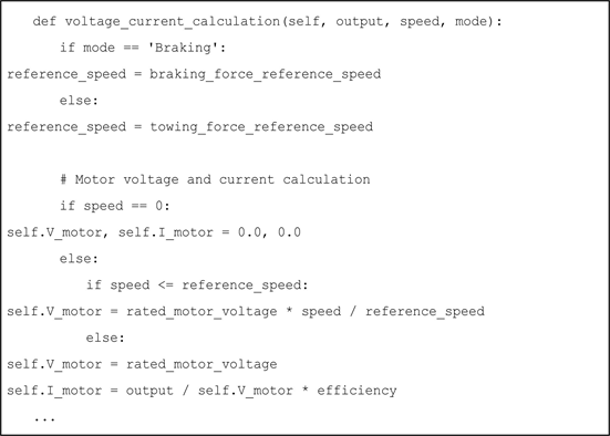
2.5. Calculation of Power Consumption and Braking Force

In the motor’s traction and braking force characteristic curve during vehicle operation, there exists a relationship between voltage change and the corresponding speed. This relationship can be obtained through Equations (5) and (6).

$F_{eff}=\{\begin{array}{ll}{V}_{dc}\times \frac{v}{v_{const}}\hfill & \left(v<v_{const}\right)\hfill \\ V\hfill & \left(v\ge v_{const}\right)\hfill \end{array}$ (5)

$I_{motor}=\frac{F\times v}{V_{motor}\times \cos \theta }\times \eta =\frac{P}{V_{motor}\times \cos \theta }\times \eta$ (6)

where:

V_motor: The motor voltage [V];

I_motor: The motor current [ton];

V_dc: The motor rated voltage [V];

v: The vehicle speed;

v_const: The reference speed for traction or braking;

F: The traction or braking force;

P: The vehicle power;

η: The traction or regeneration efficiency.

3. Object-Oriented Modeling of Railcar Propulsion

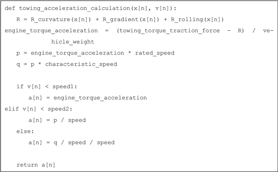
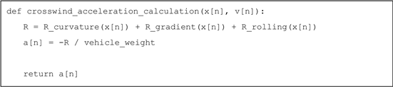
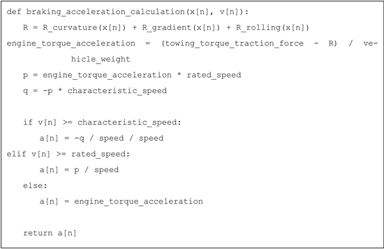
As observed, railway cars exhibit distinct kinematic characteristics within specific speed ranges. In order to capture this behavior, we outlined the construction of a vehicle motion object and demonstrated a modeling approach employing method overloading through pseudocode.

For numerical analysis of vehicle motion, we employed the fourth-order Runge-Kutta method. During the motion calculations, the form of the acceleration function varies depending on the specific speed range for traction, passing, and braking scenarios. To address this, we initially configured the acceleration calculation function, which varies based on the speed range, as follows for traction, passing, and braking.

With the aid of these acceleration calculation functions, the fourth-order Runge-Kutta function and kinematic calculation method were configured as follows.

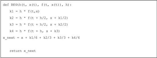
Here, the symbol f represents the derivative of x. In the subsequent motion calculation method, it is evident that the acceleration calculation function is inputted as a derivative of velocity.

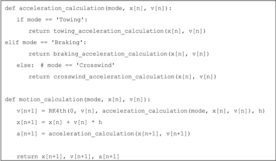
By employing function overloading, the applied acceleration function varies depending on the mode specified within the motion calculation method. Consequently, the acceleration function computes the appropriate acceleration based on the current speed range of the vehicle.

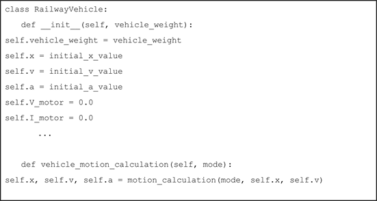
Utilizing the resulting Railcar object, one can compute the vehicle’s motion and performance within a given track environment or determine its kinematic characteristics.

4. Analyzing Vehicle Characteristics through Modeling

By utilizing the railcar object containing the computational model for the vehicle’s motion and power, we conducted simulations to compare the simulated motion with actual data. Subsequently, the vehicle model was simulated on the real track and compared against operational measurements.

4.1. Simulating Vehicle Motion and Power Characteristics

Figure 3 illustrates the time-varying speed change during reverse travel, calculated using the proposed model. In contrast, Figure 4 displays the measured data of the time-varying speed curve [8] . Notably, the vehicle maintains a consistent speed of up to 35 km/h. However, beyond this threshold, the acceleration decreases, allowing the speed to reach its maximum.

Figure 5 presents the model-calculated time-dependent curves for power usage and regenerative power, with the braking force region highlighted in red. In Figure 6, we display the measured data of the time-dependent braking force curve. Notably, the simulated braking force curve aligns with the observed electric braking force. Furthermore, it is evident that the electric braking force decreases as the air braking force, necessary for braking, gradually increases.

Through a comparison of the proposed model’s calculations of the vehicle’s speed during reverse and regenerative power during braking characteristics with the measured vehicle data, we observe that the model accurately simulates the actual characteristics of vehicle motion and power.

Figure 3. Time-dependent velocity curve (calculated).

Figure 4. Speed and other measurement data over time [8] .

Figure 5. Regenerative power curve over time (the braking region is indicated in red on the graph).

Figure 6. Braking force measurement over time [8] .

4.2. Simulating the Consumption/Regenerative Power of Train Operation

The proposed model was implemented for the Seoul Metro Line 3 to conduct TPS (Train Performance Simulation), and the obtained results were compared with the measured data [9] . Table 1 presents the vehicle specifications of the electric vehicles used as input data for TPS.

To determine the inertial mass of a train formation, the individual inertial masses of each vehicle within the formation are summed. The inertial mass of a vehicle is calculated as the sum of its curb mass, inertia factor, and passenger load. The inertia coefficient is applied to the curb mass and varies depending on whether the vehicle is an M car or a T car. For instance, let’s consider a train formation consisting of 5M5T cars, with curb weights of 39 tons for M cars and 29 tons for T cars. The inertia coefficients are 14% and 5%, respectively, and the passenger load is 20 tons per car. In this case, the inertial mass of the first formation can be calculated as follows.

Table 2 presents the speeds that delineate the constant torque and constant power regions, representing the vehicle’s acceleration and deceleration characteristics.

The constant power area spans from 35 km/h to 65 km/h for towing and 60 km/h to 75 km/h for braking.

Regarding the TPS input data, the locations of the stations are specified in Table 3.

A train operation simulation was conducted using vehicle and track data, simulating a 10-car electric train operating between Gupabal and Seoul National University of Education (Seoul University of Education). The simulation results are depicted in Figure 7.

Regarding the consumption and regeneration power of the electric vehicles on Seoul Metro Line 3, the one-way section measurement results exhibited a reverse error rate ranging from 4.03% to 8.26%, and a regeneration error rate ranging from 2.30% to 5.74%. Comparing the error rates within round-trip intervals, it was observed that the reverse error rate differed by 6.19%, while the regeneration error rate differed by 3.97%. These findings indicate that the simulation results closely estimate the actual data.

When comparing the simulation results with the actual data, a natural correspondence is observed due to the equations of motion. The peak values of regression and recovery are nearly symmetrical in the actual data. However, the peak value of power during braking appears slightly larger than the peak value during reverse. Multiplying the peak value of braking by the ratio of electric braking to air braking yields a similar value to the actual data. This characteristic is applied in actual vehicle design. Hence, it is evident that considering traction/braking efficiency and accounting for the electric braking rate would enhance the accuracy

Table 1. Vehicle specifications of an electric car as TPS input data.

Table 2. Constant torque and constant power region speeds of the vehicle.

Table 3. Locations of stations [m].

(a) (b) (c) (d)

Figure 7. Train operation energy in Gupabal to Goyang junction section. (a) Traction Energy: Gupabal → Seoul University of Education. (b) Regenerative Energy: Gupabal → Seoul University of Education. (c) Traction Energy: Seoul University of Education → Gupabal. (d) Regenerative Energy: Seoul University of Education → Gupabal.

of power values calculated through simulation for traction and braking.

5. Conclusion

In order to accurately simulate the performance of a train, it is crucial to capture the dynamics of acceleration and deceleration forces with precision. The traction and braking forces of a railroad vehicle exhibit variations depending on the speed, leading to the division of the speed range into three distinct regions: constant torque, constant power, and characteristic regions. To effectively model these characteristics, we incorporated the fourth-order Runge-Kutta method and leveraged the function overloading feature to construct vehicle objects. Employing the constructed model, we performed calculations to determine the vehicle characteristics and conducted Train Performance Simulation (TPS). By comparing the obtained results with the measured values, we validated that the model accurately represents the real-world characteristics of the vehicle.

Acknowledgements

This work was supported by the Korea Institute of Energy Technology Evaluation and Planning (KETEP) and the Ministry of Trade, Industry & Energy (MOTIE) of the Republic of Korea (No. 20225500000110).

Conflicts of Interest

The authors declare no conflicts of interest regarding the publication of this paper.

References

[1]	Kim, J.-Y. (2003) A Study on ATO Pattern for Minimizing Energy Consumption under Urban Rail System. Master’s Thesis, Seoul National University of Science and Technology, Seoul.
[2]	Kim, J.-H., Shin, H.-C., Choi, Y.-H., Han, S.-H. and Kim, L.-K. (2012) Efficient Driving Pattern of the Railway Vehicles for Driving Energy Saving. The Transactions of the Korean Institute of Electrical Engineers, 61, 1368-1373. (In Korean) https://doi.org/10.5370/KIEE.2012.61.9.1368
[3]	Lee, S.K. (2010) A Study on Optimal Design of Traction Motor Power for Urban Transit. Master’s Thesis, Hanyang University, Seoul.
[4]	Jeon, H.-J., Kim, C.-H. and Lim, J.-H. (2007) Test and Traction Characteristic of Electric Locomotives. Proceedings of the Conference of the Korean Society for Railway, Jeju, 5 May 2007, 1550-1557.
[5]	Kim, Y., Kim, S., Kim, K. and Mok, J. (2006) Study on the Deduction of Traction/Braking Forces for the Train from Acceleration/Deceleration. Journal of the Korean Society for Railway, 9, 682-688.
[6]	Choi, D., Jeon, C.S., Cho, H., Oh, H.K. and Kim, S. (2013) The Relationship between Train Weight and Acceleration for the Korea’s Next Generation Electric Multiple Unit Train. Proceedings of the Conference of the Korean Society for Railway, Daegu, 17 July 2013, 470-474.
[7]	Kim, J., Kim, M.S., Ko, K. and Jang, D.U. (2015) The Study on the Standardization of the Maximum Acceleration of the Electric Multiple Unit through the Analysis of the Traction and the Adhesion Characteristics. Journal of the Korea Academia-Industrial cooperation Society, 16, 7934-7940. (In Korean) https://doi.org/10.5762/KAIS.2015.16.11.7934
[8]	Woojin Industrial System Co. (2006) A Study on the Application of Energy Storage Technology System to Railway Stations.
[9]	Korea University (2002) Development and Application of Urban Railway Exchange Supply System Using PSCAD/EMTDC.