Complete Classical Theory of Charged Elementary Particles

Günther Landvogt

Independent Researcher, Hamburg, Germany.

DOI: 10.4236/jhepgc.2023.93061                

Abstract

Electron, proton, and their antiparticles consist of an electromagnetic field and a constituent that creates it. The simplest constituent is a one-dimensional circular current loop. The elementary charge is homogeneously distributed over its circumference and rotates at a constant velocity. The charge creates an electrostatic field. Its rotation represents a current that creates a magnetic field. Balance between the electric and magnetic forces ensures stability. This requires a marginal radial extension of the loop that makes the particle two-dimensional. In the near vicinity of two equal concentric current loops the axial attractive magnetic force compensates for the axial repelling electrostatic force. This discovery explains the weak (electron) and strong (proton) nuclear forces. Electron and proton have normal magnetic moments. The measured “anomalies” indicate the existence of a hidden rotational kinetic energy caused by rotation of the annular particle mass. So, there are four natural forces: electric, magnetic, kinetic, and gravitational. This knowledge makes the search for the Grand Unified Theory (GUT) trivial. The discovered rotational energy affects Einstein’s and Planck’s energy equations and leads to the exact calculation of the Lamb shifts and the binding energies of the hydrogen-like atoms. The theory predicts stable multiple particles and explains the Cooper Pair. For the first time the Planck mass and the gravitational constant are analytically calculated at high accuracy.

Keywords

Natural Forces, Magnetic Moment, Lamb Shift, Rotational Energy, Gravitational Constant

1. Introduction

Since more than hundred years it is well-known that electron and proton (besides the neutron) are the most important building blocks of matter. As they are stable and cannot be divided into smaller particles, they are called elementary. There are only four such particles: Electron, proton, positron, and antiproton. They are characterized by the following four basic entities:

Elementary charge $\pm e$ anomaly of magnetic moment $a_e$ , $a_p$

rest mass $m_0$ angular momentum $\hslash /2$

Up to now the knowledge about their internal structure is poor and confusing. Strange but true: As electron and positron seem to show no internal structure, quantum physics regards them as point particles having no dimensions at all. Such an object is totally unrealistic and non-physical. It cannot have any physical properties: Charge density and mass density would be infinite, angular momentum, magnetic flux, and magnetic moment could not exist. Proton and antiproton are regarded as small spherical objects consisting of up and down quarks with rather strange, contradictory properties. It will be shown that classical physics does not need such complicated models.

The first serious approach to a physical theory of the electron, published in 1990 by Bergman and Wesley [1] is based on a toroidal ring with uniformly distributed charge. In 2018 Consa [2] used the same principle for a modified and extended electron model. The presented article is based on an independent publication of the author [3] that is hidden in the web since 2014. It proposes a circular current loop as a particle model and derives from it the complete set of mathematical formulas to calculate exactly the electric and magnetic energies and forces. Moreover, the existence of a rotational kinetic energy was predicted that removed the “anomaly” of electron’s magnetic moment. The results were encouraging, but some conclusions were provisional and will be revised and extended here. Especially the nature of the strange magnetic moment anomaly of the proton will be explained. Parson [4] recommended the current loop model “…proposing that the unit negative charge is distributed continuously around the ring…” already in 1915. It would have been the right idea to improve Bohr’s well-known model of the hydrogen atom and thus to avoid modern quantum electrodynamics (QED).

2. The Circular Current Loop

First it is postulated that a charged elementary particle consists of its electromagnetic field and of a constituent that creates it. A one-dimensional circular current loop having a finite radius R and carrying the elementary charge $\pm e$ is the simplest object that can serve as the field-generating constituent. The most important idea is that the elementary charge $\pm e$ is distributed homogeneously over its circumference $2\pi R$ and that it rotates at a constant velocity $v_c$ . These are the conditions for the existence of a constant current and a constant magnetic field in addition to the constant electrostatic field of the charge. To be stable the concerned charged particles must generate a constant centripetal magnetic force being in balance with the centrifugal force of the charge. This is the only chance that the model can represent a stable, non-radiating particle. Expressed in terms of James Clerk Maxwell it means

$\frac{\partial B}{\partial t}=0$ (2.1)

where B is the density of the magnetic flux $\varphi$ . Thus, the particles under investigation will be a special solution to Maxwell’s equations. But the solution doesn’t describe any kind of a wave, but it is a simple direct current system representing an elementary magnet.

The direction of the current defines its North Pole and front side (Figure 1). Viewed from the rear side (South Pole) the current shows the opposite direction (mirror image, reverse clock). The presented particle model demonstrates that there are not two kinds of a loaded elementary particle, indicated by a positive respectively negative spin. The spin quantum number is not necessary and misleading. There is no intrinsic spin, but only a normal angular momentum. The particle has a constant electric field resulting from the distributed charge and a constant magnetic field resulting from the rotation of the distributed charge at a constant velocity $v_c$ . The two most important—and rather demanding—tasks are to find the scalar potential function V describing the electrostatic field and the vector potential $A$ describing the magnetic field. The results are needed to calculate the electric and magnetic energies and the respective forces. This is already done in [3] and will be used below.

3. Electric and Magnetic Energies

In [3] the investigation on the energies started at the statement that the (inertial) energy $E_0=m_0{c}^2$ consists of the electric energy $E_{el}$ and the magnetic energy $E_{mag}$ :

$E_{el}+E_{mag}=\left(m_{el}+m_{mag}\right)c^2=m_0{c}^2$ (3.1)

The surprising result of the energy calculations in [3] is

$E_{el}-E_{mag}=m_0{c}^2\frac{\alpha }{2\pi }\frac{{ƛ}_C}{R}$ (3.2)

Figure 1. One-dimensional circular current loop.

where the velocity $v_c$ of the rotational charge is provisionally supposed to be c, the velocity of light:

$v_c=c\cdot {\beta }_c=c$ (3.3)

From (3.1) and (3.2) follows

$E_{el}=\frac{1}{2}{m}_0{c}^2\left(1+\frac{{ƛ}_C}{R}\frac{\alpha }{2\pi }\right)$ (3.4)

and

$E_{mag}=\frac{1}{2}{m}_0{c}^2\left(1-\frac{{ƛ}_C}{R}\frac{\alpha }{2\pi }\right)$ (3.5)

These results are already found in [1] , where a toroidal electron model was used. When particle physics is based on point particles, such a result can never be found, because magnetic energy doesn’t exist and consequently cannot be correctly calculated. The electrical energy arises from the distributed charge and its electrostatic field. As already stated in [1] , it is purely static and cannot contribute to dynamic effects such as magnetic flux, magnetic moment, angular momentum, and rotational impulse. These effects arise exclusively from the current represented by the rotating, homogeneously distributed charge. From the statement (3.5), the assumption (3.3), and the knowledge of the commonly accepted value of the angular momentum is

$m_{mag}{v}_{c}R=\frac{1}{2}{m}_0\left(1-\frac{{ƛ}_C}{R}\frac{\alpha }{2\pi }\right)cR=\frac{1}{2}\hslash$ (3.6)

The resulting radius R is (provisionally)

$R={ƛ}_C\left(1+\frac{\alpha }{2\pi }\right)$ (3.7)

with the radius of (3.7) the energy Equations (3.4) and (3.5) become

$E_{el}=\frac{1}{2}{m}_0{c}^2\left(1+\frac{\frac{\alpha }{2\pi }}{1+\frac{\alpha }{2\pi }}\right)=\frac{1}{2}{m}_0{c}^2\left(1+a\right)$ (3.8)

$E_{mag}=\frac{1}{2}{m}_0{c}^2\left(1-\frac{\frac{\alpha }{2\pi }}{1+\frac{\alpha }{2\pi }}\right)=\frac{1}{2}{m}_0{c}^2\left(1-a\right)$ (3.9)

The constant

$a=\frac{\frac{\alpha }{2\pi }}{1+\frac{\alpha }{2\pi }}=1.160062425\cdots \times {10}^{-3}$ (3.10)

is slightly different from the measured “anomaly” $a_e$ of electron’s the magnetic moment [5] :

$a_e=1.15965218128\times {10}^{-3}$ (3.11)

The constant $a\approx a_e$ turns out as a universal parameter that is crucial for the theory of charged elementary particles. The statements (3.6) and (3.7) will be corrected later-on, but the Equations (3.8), (3.9), and (3.10) will remain unchanged.

4. Rotational Kinetic Energy, Total Mass/Energy

In [3] the interpretation of $a_e$ as an “anomaly” of the magnetic moment $\mu$ of the electron is proved to be erroneous. As the magnetic moment is due to the current $I_{\phi }$ in $\phi$ direction the result should be related to the mass $m_{\phi }$ in $\phi$ direction rather than to the rest mass $m_0$ . So, what really is measured is

$\mu =\frac{e\hslash }{2m_{\phi }}\left(1+a_e\right)$ (4.1)

The difference between $m_{\phi }$ and $m_0$ is interpreted as an additional rotational kinetic energy:

$E_{rot}=m_0{c}^2{a}_e$ (4.2)

with the assumption

$m_{\phi }=m_0\left(1+a_e\right)$ (4.3)

the true magnetic moment becomes

$\mu =\frac{e\hslash }{2m_{\phi }}\left(1+a_e\right)$ (4.4)

From now Special Relativity is involved. The “anomaly” subject is investigated more deeply in chapter 7.

Total consistency of the presented theory is achieved when the magnetic energy $E_{mag}$ is supported by adding the kinetic rotational energy $E_{rot}$ according to (4.2). Van de Togt [6] has proven the equivalence of magnetic and kinetic energy. So, it is natural to treat them together. There are two alternatives how nature might generate $E_{rot}$ :

The rotational kinetic energy $E_{rot}$ may be created by rotation of the inertial mass $m_0$ :

$E_{rot}=m_0{c}^2\left(\frac{1}{\sqrt{1-{\beta }_m^2}}-1\right)=m_0{c}^2\cdot a$ (4.5)

The rotational velocity

$v_m=c\cdot {\beta }_m$ (4.6)

of the magnetic mass $E_{mag}/c^2$ can be calculated from (4.5):

$\frac{1}{\sqrt{1-{\beta }_m^2}}=1+a$ (4.7)

and finally

${\beta }_m=\frac{v_m}{c}=\frac{\sqrt{a\left(2+a\right)}}{1+a}=\text{0}\text{.048125813}\cdots$ (4.8)

Alternatively, the kinetic energy could be created by rotation of the magnetic mass according to (3.9)

$E_{rot2}=\frac{1}{2}{m}_0{c}^2\left(1-a\right)\left(\frac{1}{\sqrt{1-{\beta }_{m2}^2}}-1\right)=m_0{c}^2\cdot a$ (4.9)

The rotational velocity

$v_{m2}=c\cdot {\beta }_{m2}$ (4.10)

of the magnetic mass $E_{mag}/c^2$ can be calculated from (4.9):

$\frac{1}{\sqrt{1-{\beta }_{m2}^2}}=1+\frac{2a}{1-a}$ (4.11)

and finally

${\beta }_{m2}=\frac{2\sqrt{a}}{1+a}=0.068040447\cdots$ (4.12)

The author’s research on the hydrogen atom brought the discovery, that the kinetic rotational energy is the origin of the Lamb shift. The decision between the two alternatives is given by the fact that the Lamb shift theory with ${\beta }_m$ fits the experimental results, but it fails with ${\beta }_{m2}$ .

This means that the inertial masses $m_0$ of charged elementary particles rotate (as a whole) at the velocity

$v_m={\beta }_m\cdot c=\frac{\sqrt{a\left(2+a\right)}}{1+a}\cdot c$ (4.13)

and contribute to their angular momentum. Macroscopic bodies (astronomy!) generally possess a rotational energy, too, but it is arbitrary and not bound to their inertial mass by a fixed factor.

According to (3.8) the electric energy remains

$E_{el}=\frac{1}{2}{m}_0{c}^2\left(1+a\right)$ (4.14)

The sum of $E_{mag}$ according to (3.9) and $E_{rot}$ according to (4.5) is the dynamic energy

$E_{dyn}=E_{mag}+E_{rot}=\frac{1}{2}{m}_0{c}^2\left(1+a\right)=E_{el}$ (4.15)

The symmetry established by $E_{dyn}=E_{el}$ corresponds to the fact that with electromagnetic waves the electric energy is equal to the magnetic energy.

Due to the relativistic contribution $E_{rot}$ charged elementary particles can no longer be considered as pure electromagnetic objects! Besides Maxwell’s theory Einstein’s Special Relativity is involved.

Surprisingly the total particle energy $E_{total}$ of charged elementary particles is

$E_{total}=E_{el}+E_{mag}+E_{rot}=m_0{c}^2\left(1+a\right)$ (4.16)

Einstein’s inertial energy $E_0=m_0{c}^2$ is increased by the hidden rotational kinetic energy

$E_{rot}=m_0{c}^{2}a$ (4.17)

Thus, the electron possesses the rotational energy

$E_{rot,e}=m_0{c}^{2}a=\text{592}\text{.6}\text{eV}$ , (4.18)

The respective value of the proton is

$E_{rot,p}=m_{p,0}{c}^{2}a=1.088\text{MeV}$ (4.19)

The relativistic mass increase cannot be measured by acceleration or gravitational experiments. The relativistic effect resulting in $m_{\phi }=m_0\left(1+a\right)$ is due to rotation in radial direction $\phi$ and, according to Special Relativity, does not affect the physical situation in other directions. Of course, this only holds when the radius of the respective particle is constant during the experiments, i.e. when the experiments concern free particles.

One of the important consequences of (4.16) is the impact on Planck’s energy equation

$E=hf=\frac{hc}{\lambda }=\frac{\hslash c}{{ƛ}_C}$ (4.20)

where

$\frac{\hslash c}{{ƛ}_C}=\hslash c\cdot \frac{m_{0}c}{\hslash }=m_0{c}^2$ (4.21)

So, Planck’s photon energy, being Planck’s constant h multiplied by the frequency f, matches exactly Einstein’s inertial energy:

$E_0=hf=m_0{c}^2$ (4.22)

This was the logical intention when Planck’s constant was defined. But according to (4.16) the total particle energy is

$E_{total}=m_0\left(1+a\right)\cdot c^2=h\left(1+a\right)\cdot f$ (4.23)

The discovered rotational kinetic energy is a necessary step for the development of the Grand Unified Theory (GUT). It is crucial when a photon creates an electron and a positron (pair production): The photon must spend the total energy $2\cdot E_{total}$ of the particle pair. This important effect is used in chapter 10, where the correct formula of the Lamb shift is derived, and in chapter 11, where the Planck mass and the gravitational constant are analytically calculated.

The rotation of the total particle mass according to (4.3) at the velocity according to (4.13) causes the centrifugal force

$F_{fug}=\frac{m_0\left(1+a\right)c^2}{r}\cdot \frac{a\left(2+a\right)}{{\left(1+a\right)}^2}$ (4.24)

The electric force is

$F_{el}=\frac{e^2}{4\pi {\epsilon }_0}\cdot \frac{1}{r^2}=\frac{\alpha \hslash c}{r^2}$ (4.25)

where

$r=ƛ=\frac{\hslash }{m_{0}c}$ (4.26)

Thus, the ratio

$\frac{F_{fug}}{F_{el}}=\frac{2a}{\alpha }\cdot \frac{1+a/2}{1+a}$ (4.27)

doesn’t depend on the particle radius and is the same for the electron and the proton. Regarding (3.10)

$\frac{F_{fug}}{F_{el}}\approx \frac{1}{\pi }$ (4.28)

But relevant for the force balance are the force differences

$\text{Δ}{F}_{el}=\frac{\alpha \hslash c}{r_1^2-r_2^2}\approx \frac{\alpha \hslash c}{r_1^2\cdot 2{\delta }_r}$ (4.29)

and

$\text{Δ}{F}_{fug}=\frac{\frac{1}{2}{m}_0\left(1+a\right){\delta }_r{c}^2}{r_1{\delta }_r}\cdot \frac{a\left(2+a\right)}{{\left(1+a\right)}^2}\cdot 2{\delta }_r$ (4.30)

where according to (8.12)

${\delta }_r\approx 2.470\times {10}^{-4}$ (4.31)

Thus, the influence of the centrifugal force on the properties of the particle is given by

$\frac{\text{Δ}{F}_{fug}}{\text{Δ}{F}_{el}}\approx \frac{1}{\pi }\cdot {\delta }_r^2\approx 2.32\times {10}^{-8}$ (4.32)

The effect is too small to improve the results of the theory essentially, but it should be worth to mention it.

5. Charge Velocity, Radius, Angular Momentum

In [3] the radial electric force and the radial magnetic force are calculated. Essential result: When the charge velocity

$v_c=\sqrt{v_{\phi 1}{v}_{\phi 2}}={\beta }_{c}c$ (5.1)

is assumed to be c, the velocity of light, the calculated radial magnetic force slightly exceeds the calculated radial electric force. This is valid in the total range $0<r_2/r_1<1$ . At this condition the respective particle would be unstable at any choice of $r_2/r_1$ . Force balance exists when

${\beta }_c^2{F}_{mag,radial}=F_{el,radial}$ (5.2)

Numerical results: Depending on the choice of $r_2/r_1$ force balance can be established for any value of

${\beta }_c^2\le 0.9996628$ (5.3)

The limiting value

${\beta }_{c,\max }=\text{0}\text{.9998314}$ (5.4)

is reached at

${\frac{r_2}{r_1}|}_{\max }=0.9999787=1-2.13\times {10}^{-5}$ (5.5)

when $r_2/r_1$ is smaller than this maximum attainable value, ${\beta }_c$ is smaller than ${\beta }_{c,\max }$ and the force balance results in a stable particle. Conversely, at higher values of $r_2/r_1$ , where the charge velocity drops down to zero at

${\beta }_c\approx 1-5\times {10}^{-9}$ (5.6)

stable particles don’t exist. (These results are calculated at $n_{\max }=3\times {10}^9$ steps of the two radial force series.)

The existence of the rotational kinetic energy according to (4.5) makes the provisional statement (3.7) for the radius R obsolete. The new knowledge of $E_{dyn}$ according to (4.15) leads to the angular momentum

$m_{dyn}\cdot v_c\cdot R=\frac{1}{2}{m}_0\left(1+a\right)\cdot v_c\cdot R=\frac{\hslash }{2}$ (5.7)

and

$\left(1+a\right)\cdot \frac{v_c}{c}\cdot R=\frac{\hslash }{m_{0}c}={ƛ}_C$ (5.8)

As already mentioned in chapter 3, the electric energy $E_{el}$ respectively its equivalent mass $E_{el}/c^2$ do not contribute to the angular momentum of stable charged particles.

As the charge velocity

$v_c=\sqrt{v_{\phi 1}{v}_{\phi 2}}$ (5.9)

is expected to be slightly below c, the only reasonable consequences can be

$R={ƛ}_C=\frac{\hslash }{m_{0}c}=3.8615926796\times {10}^{-13}\text{m}$ (5.10)

$\frac{v_c}{c}=\frac{1}{1+a}=0.998841282760$ (5.11)

The radius $R={ƛ}_C$ of the field-generating current loop of a stable charged particle is inversely proportional to the inertial (rest) mass $m_0$ . Bergman and Wesley [1] found this basic law already in 1990.

The common interpretation of angular momentum measurements is

$m_0\cdot c\cdot R=\frac{\hslash }{2}$ (5.12)

It is irritating: From the definition of fine structure constant

$\alpha =\frac{e^2}{4\pi {\epsilon }_0\cdot \hslash c}$ (5.13)

should be clear and generally accepted that fractional values of the angular momentum in nature cannot occur because fractional values of $\pm e$ are not observed. When a photon transporting the energy $\ge 2\cdot m_0{c}^2\left(1+a\right)$ and the angular momentum $\hslash$ is split up into an electron and a positron, each having the total energy $E_{total}=m_0{c}^2\left(1+a\right)$ , the electrostatic half of the two particles doesn’t get any angular momentum at all, whereas the dynamic masses $m_{dyn}=m_{total}/2$ of the two particles share the angular momentum of the photon. According to (5.10) and (5.11) is

$\frac{1}{2}J=\frac{1}{2}{m}_0\left(1+a\right)\cdot \frac{c}{1+a}\cdot \frac{\hslash }{m_{0}c}=\frac{1}{2}\hslash$ (5.14)

Thus, the two created particles don’t have the impossible angular momentum $\hslash /2$ , but, as a matter of correct physical association, the full angular momentum $J=\hslash$ each. So, (5.7) also represents the angular momentum of the complete particle:

$m_{total}\cdot v_c\cdot R=\hslash$ (5.15)

The calculation of the correct particle parameters starts with the conditions

${\left(\frac{v_c}{c}\right)}^2=\frac{1}{{\left(1+a\right)}^2}=0.997683906149$ (5.16)

and

$\frac{1}{{\left(1+a\right)}^2}{F}_{mag,radial}=F_{el,radial}$ (5.17)

The respective value of $r_2/r_1$ is found by iteration. The result is

$r_2/r_1=0.999752965562932=1-{\delta }_e$ (5.18)

${\delta }_e=2.47034437067972\times {10}^{-4}$ (5.19)

Compared to (5.11) the charge velocity $v_{c,e}=c{\beta }_{c,e}$ of the electron, derived from the experimental “anomaly” $a_e$ according to (3.11) is

${\beta }_{c,e}=\frac{1}{1+a_e}=0.998841691$ (5.20)

6. Current, Magnetic Flux, Additional Entities

The current I of a circular current loop of radius R is generally

$I=\frac{e{v}_c}{2\pi R}=\frac{ec}{2\pi R}\cdot {\beta }_c$ (6.1)

According to (5.11) is

$v_c=\frac{c}{1+a}$ (6.2)

and according to (5.10)

$R={ƛ}_C=\frac{\hslash }{m_{0}c}$ (6.3)

Consequently is

$I=\frac{e}{2\pi \hslash }\frac{m_0{c}^2}{1+a}=\frac{e}{h}\frac{m_0{c}^2}{1+a}$ (6.4)

Just to give an impression of the huge amounts: The electron current $I_{el}$ is

$I_{el}\approx 19.773\text{A}$ (6.5)

The proton current $I_{pr}$ is

$I_{pr}\approx 36307\text{A}$ (6.6)

The magnetic flux $\Phi =L\cdot I$ can be found by means of the inductance L and the magnetic energy:

$E_{mag}=\frac{1}{2}L{I}^2$ (6.7)

It must be equal to the magnetic energy according to (3.9):

$E_{mag}=\frac{1}{2}{m}_0{c}^2\left(1-a\right)=\frac{1}{2}L{I}^2$ (6.8)

Together with the current according to (6.4) it allows to calculate the magnetic flux $\Phi$

$\Phi =L\cdot I=\frac{m_0{c}^2\left(1-a\right)}{I}=m_0{c}^2\left(1-a\right)\frac{2\pi \hslash }{e}\frac{1+a}{m_0{c}^2}$ (6.9)

The interesting result is

$\Phi =\frac{2\pi \hslash }{e}\left(1-a^2\right)=\frac{h}{e}\left(1-a^2\right)$ $a^2\approx 1.3\times {10}^{-6}$ (6.10)

The magnetic flux $\Phi \approx h/e$ is a basic entity at the same physical importance level as the elementary charge e. The point particle physics doesn’t know magnetic flux, but $\Phi \approx h/e$ is common to all charged elementary particles such as electron and proton and their antiparticles.

From (6.4) and (6.7) the inductance L can be calculated:

$L={\left(\frac{h}{e}\right)}^2\frac{{\left(1+a\right)}^2}{m_0{c}^2}\left(1-a\right)=\frac{{\mu }_0}{2\alpha }{\lambda }_C{\left(1+a\right)}^2\left(1-a\right)$ (6.11)

Analogously the capacitance C can be calculated from the electric energy

$E_{el}=\frac{1}{2}C{U}^2=\frac{1}{2}{m}_0{c}^2\left(1+a\right)$ (6.12)

and the charge condition

$Q=e=CU$ (6.13)

The result is

$C=\frac{e^2}{m_0{c}^2\left(1+a\right)}=2\alpha {\epsilon }_0{\lambda }_C\frac{1}{1+a}$ (6.14)

Furthermore is

$\frac{1}{\sqrt{LC}}=\frac{m_0{c}^2}{h}\frac{1}{\sqrt{1-a^2}}=\frac{c}{{\lambda }_C}\frac{1}{\sqrt{1-a^2}}$ (6.15)

and

$\sqrt{\frac{L}{C}}=\frac{h}{e^2}\left(1+a\right)\sqrt{1-a^2}=\frac{1}{2\alpha }\sqrt{\frac{{\mu }_0}{{\epsilon }_0}}\left(1+a\right)\sqrt{1-a^2}$ (6.16)

Inductance, capacitance and their two combinations are not essential for the presented theory, because the field-generating circular loop is a direct current circuit. But they are clearly defined and belong to physical reality. They may be helpful or necessary for further research.

7. Magnetic Moment and Landé Factor

The definition of the magnetic moment of a circular current loop with the current I and the radius R is

$\mu =I\pi R^2$ (7.1)

when the homogenously distributed elementary charge e rotates at the velocity v around the circumference $2\pi R$ , the current is

$I=\frac{ev}{2\pi R}$ (7.2)

It creates the magnetic moment

$\mu =\frac{ev}{2}R$ (7.3)

The angular momentum is

$mvR=\hslash$ (7.4)

with

$vR=\frac{\hslash }{m}$ (7.5)

as generally assumed, the magnetic moment results in

$\mu =\frac{e\hslash }{2m_0}$ (7.6)

This is only valid with non-rotating objects where the relativistic mass increase, caused by rotation, is missing. As the magnetic moment is caused by a current flowing in $\phi$ direction, for the calculation of $\mu$ the mass $m_{\phi }=m_0\left(1+a\right)$ must be used. Conversely, measurements of the magnetic moment are perhaps the unique opportunity to measure the universal constant $a$ .

When the magnetic moment of the electron is measured, the experimental result is interpreted as

${\mu }_e=\frac{e\hslash }{2m_{e0}}\left(1+a_e\right)$ (7.7)

But what really is measured is

${\mu }_e=\frac{e\hslash }{2m_{e0}\left(1+a\right)}\left(1+a_e\right)$ (7.8)

when the values according to (3.10) and (3.11) are inserted, the theoretic result is

${\mu }_e=\frac{e\hslash }{2m_{e0}}\cdot \left(1-4.097688\times {10}^{-7}\right)$ (7.9)

The theory presented here requires the pleasant result

${\mu }_e=\frac{e\hslash }{2m_{e0}}={\mu }_B$ (7.10)

where ${\mu }_B$ is the Bohr magneton.

What about the “exotic” proton? How can its huge “anomaly” $a_p^{\ast }\approx 1.79$ be explained?

Analogously to (7.8) the magnetic moment ${\mu }_p$ of the proton might be expected to be

${\mu }_p=\frac{e\hslash }{m_{p,0}\left(1+a\right)}\left(1+a_p^{\ast }\right)$ (7.11)

where

$a_p^{\ast }=1.79284734463$ (7.12)

is the carefully measured value [5] of its “anomaly”. But the evaluation of the measurement is based on the incorrect interpretation

${\mu }_p=\frac{e\hslash }{2m_{p,0}}\left(1+a_p^{\ast }\right)$ (7.13)

Compared to the electron there is a significant difference: According to the presented theory the magnetic moment of the proton should be regular, too. This means that it should be $a_p^{\ast }=1+a$ . The situation is easy to explain: Compared to the electron the rotational energy of the proton is proportional to the mass while the magnetic moment is inversely proportional to the mass. What has happened is that in (7.12) the constant a appears erroneously multiplied by the factor ${\mu }_p/{\mu }_e=m_{p,0}/m_{e,0}$ such that this factor is included in the measurement of $a_p^{\ast }$ . What really is measured is

${\mu }_p=\frac{e\hslash }{2m_{p,0}\left(1+a\right)}\left(1+\frac{m_{e,0}}{m_{p,0}}\cdot a_p^{\ast }\right)$ (7.14)

where

$a_p=\frac{m_{e,0}}{m_{p,0}}\cdot a_p^{\ast }=9.764151808\times {10}^{-4}$ (7.15)

and

$\frac{a_p}{1+a}=9.752837907\times {10}^{-4}$ (7.16)

The theoretical result should be $a_p=a_e\approx a$ . Thus, the magnetic moment of the proton, based on the measured “anomaly” $a_p^{\ast }$ deviates slightly from the expected theoretical value:

${\mu }_p=\frac{e\hslash }{2m_{p,0}}\left(1-1.834346\times {10}^{-4}\right)\approx \frac{e\hslash }{2m_p}$ (7.17)

There is high evidence that the magnetic moment ${\mu }_p$ of the proton is equal to the nuclear magneton ${\mu }_N$ :

${\mu }_p={\mu }_N=\frac{e\hslash }{2m_{p,0}}$ (7.18)

The Equations (7.9) and (7.17) demonstrate that the magnetic moment $\mu$ of charged elementary particles is generally

$\mu =\frac{e\hslash }{2m_0}$ (7.19)

It is the same as in classical physics. According to (5.14) the angular momentum is $\hslash$ . So, the gyromagnetic ratio $\gamma$ is quite regularly

$\gamma =\frac{\text{magnetic}\text{moment}}{\text{angular}\text{momentum}}=\frac{q}{2m}=\frac{e}{2m_0}$ (7.20)

as it is with a classical slowly rotating body having the charge $q=e$ and the rest mass $m=m_0$ .

The Landé factor is always

$g=1$ (7.21)

and has become a trivial entity.

8. Weak and Strong Nuclear Forces

In [3] six formulas based on classical Potential Theory are derived. They describe the electric and magnetic energies and forces of the circular current loop model. In this chapter two of them concerning the axial electric force $F_{elz}\left(r_2,z\right)$ and the axial magnetic force $F_{magz}\left(r_2,z\right)$ between two charged particles are repeated and adapted:

$F_{elz}\left(r_2,z\right)=\frac{\alpha \hslash c}{r_1^2}\frac{q_1}{e}\frac{q_2}{e}\frac{{\displaystyle \underset{n=0}{\overset{\infty }{\sum }}{a}_{2n}\left(4n+1\right)k^{2n}}}{{\left[1+{\left(\frac{r_2}{r_1}\right)}^2+{\left(\frac{z}{r_1}\right)}^2\right]}^{\frac{3}{2}}}\frac{z}{r_1}$ (8.1)

$F_{magz}\left(r_2,z\right)=-\frac{\alpha \hslash c}{r_1^2}\frac{q_1}{e}\frac{q_2}{e}\frac{v_{\phi 1}}{c}\frac{v_{\phi 2}}{c}\frac{{\displaystyle \underset{n=0}{\overset{\infty }{\sum }}{b}_{2n}\left(n+\frac{3}{4}\right)k^{2n+1}}}{{\left[1+{\left(\frac{r_2}{r_1}\right)}^2+{\left(\frac{z}{r_1}\right)}^2\right]}^{\frac{3}{2}}}\frac{z}{r_1}$ (8.2)

The coefficient k is

$k=\frac{2\frac{r_2}{r_1}}{1+{\left(\frac{r_2}{r_1}\right)}^2+{\left(\frac{z}{r_1}\right)}^2}$ (8.3)

The coefficients $a_{2n}$ and $b_{2n}$ are

$a_0=1$ $a_{2n}=a_{2n-2}\cdot \frac{4n-1}{4n}\cdot \frac{4n-3}{4n}$ (8.4)

$b_0=1$ $b_{2n}=b_{2n-2}\cdot \frac{4n-1}{4n}\cdot \frac{4n+1}{4n+4}$ (8.5)

These common equations describe the mutual axial forces between two concentric circular current loops as a function of their relative distance $z/r_1$ and the ratio $r_2/r_1$ of their radii. Their charges are $q_1$ and $q_2$ , and their rotational charge velocities are $v_{\phi 1}$ and $v_{\phi 2}$ . The velocities are related to c, the velocity of light. To synthesize an electron, in [3] the special, idealized case

$q_1=q_2=\pm e/2$ (8.6)

$r_2=r_1$ (8.7)

$v_{\phi 1}=v_{\phi 2}=c$ (8.8)

is treated. One goal was to prove the stability of the electron by finding the force balance conditions between the centrifugal electric force and the centripetal magnetic force at $z/r_1=0$ where both current loops are concentrically positioned in the same plain. The result of the numerical calculation was that at condition (8.8) the centripetal magnetic force is slightly higher (!) than the centrifugal electric force. So, force balance requests $v_{\phi 1}=v_{\phi 2}<c$ and is fulfilled by (8.9), (8.10), and (8.11)

$v_c=\frac{c}{1+a}$ (8.9)

$r_1={ƛ}_C\left(1+a\right)$ (8.10)

$\frac{r_2}{r_1}=1-{\delta }_r$ (8.11)

The calculated value of ${\delta }_r$ is

${\delta }_r=2.47034437067972\times {10}^{-4}$ (8.12)

A stable electron according to the current loop model is a two-dimensional object. It needs a small radial expansion represented by two concentric, slightly different current loops, each carrying the (nonphysical) charge $-e/2$ . Generally: Charged elementary particles are two-dimensional! The presented theory does not require the axial dimension. In (8.14), (8.15), and (8.16) the updated results of (8.9), (8.11), and (8.12) are considered. When in chapter 4 the magnetic energy had to be introduced into the theory, (8.10) had to be corrected to

$r_1=R={ƛ}_C$ (8.13)

according to (5.10). Besides the inertial mass $m_0$ the total mass

$m_0=m_0\left(1+a\right)$ (8.14)

and besides the inertial energy $E_0=m_0{c}^2$ the total energy

$E_{total}=m_0{c}^2\left(1+a\right)$ . (8.15)

had to be introduced. When (8.1) and (8.2) are specialized to

$r_2\approx r_1=R={ƛ}_C$ (8.16)

and

$q_1=q_2=\pm e$ (8.17)

they describe the mutual electric and magnetic forces of two equal, stable, charged elementary particles as a function of their axial distance. Their force equations derived from (8.1) and (8.2) are

$F_{elz}\left(\frac{z}{{ƛ}_C}\right)=\frac{\alpha \hslash c}{{ƛ}_C^2}\frac{{\displaystyle \underset{n=0}{\overset{\infty }{\sum }}{a}_{2n}\left(4n+1\right)k^{2n}}}{{\left[2-{\delta }_r+{\left(\frac{z}{{ƛ}_C}\right)}^2\right]}^{\frac{3}{2}}}\frac{z}{{ƛ}_C}$ (8.18)

and

$F_{magz}\left(\frac{z}{{ƛ}_C}\right)=-\frac{\alpha \hslash c}{{ƛ}_C^2}\frac{1}{{\left(1+a\right)}^2}\frac{{\displaystyle \underset{n=0}{\overset{\infty }{\sum }}{b}_{2n}\left(n+\frac{3}{4}\right)k^{2n+1}}}{{\left[2-{\delta }_r+{\left(\frac{z}{{ƛ}_C}\right)}^2\right]}^{\frac{3}{2}}}\frac{z}{{ƛ}_C}$ (8.19)

where

$k=\frac{2\left(1-{\delta }_r\right)}{2-{\delta }_r+{\left(\frac{z}{{ƛ}_C}\right)}^2}$ (8.20)

Compared to [3] , where the charges were chosen according to (8.6), all forces are increased by the factor 4, because the charges $q_1$ and $q_2$ now have the physically correct values according to (8.17). At relative distances $z/R=z/{ƛ}_C>3$ between the two current loops the amount of the attractive magnetic force (blue curve) is much smaller than the repulsive electric force (red curve) as shown in Diagram 1. At distances $z/R={ƛ}_C<0.3$ the magnetic force and the electric force are nearly equal. The green curve shows their small difference. At

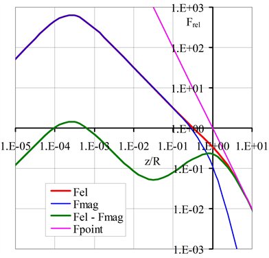
Diagram 1. Related axial forces $F/\left(\alpha \hslash c/{ƛ}_C^2\right)$ of two real particles as a function of their relative distance $z/R=z/{ƛ}_C$ .

$z_M/R\approx 3\times {10}^{-4}$ their values, related to the force $F/\frac{\alpha \hslash c}{{ƛ}_C^2}$ , arrive at a maximum of ≈800 and then drop down to zero at $z_0/R=0$ .

The two concentric current loops in axial direction are in force balance when both are positioned at $z_0/R=0$ in the same plane. No additional forces are needed to “glue” two equal particles together, when they are brought concentrically to the same axial position. Of course, the current of the particles must have the same direction. Otherwise, both the electric and the magnetic forces would have the same sign, and it would be impossible to bring them together.

The $F_{point}$ curve shows the respective (hypothetical) behavior of two point- particles. Such particles cannot exist, because their repulsive electric force could not have a compensating counterpart and thus would become infinity at $z_0/R=0$ . When the nonsensical assumptions of point particles and point charges are maintained, it is necessary to invent something that brings the absurd theory in accordance with experience. The two inventions are the “strong” nuclear force for interacting protons and the “weak” nuclear force for interacting electrons. It is not necessary to invent these two “fundamental interactions”. The job is done quite naturally and perfectly by the magnetic forces of the concerned particles. The magnetic force is a natural force for its own besides the electric force and gravity. The centrifugal, too, is obviously a natural force. Its (small) influence was not investigated so far.

The search for a Grand Unified Theory (GUT) that unifies the “electro­magnetic interaction”, the “strong nuclear force”, and the “weak nuclear force” has found a trivial end. The integration of gravity will be a hard job, but a small step in this direction is already done in chapter 11.

The Equations (8.18) and (8.19) show that the electric and magnetic forces are inversely proportional to ${ƛ}_C^2$ . So, the ratio of the weak and strong forces is the ratio between the magnetic forces of the electron and the proton and can easily be calculated:

$\frac{F_{weak}}{F_{strong}}={\left(\frac{{ƛ}_{Cproton}}{{ƛ}_{Celectron}}\right)}^2={\left(\frac{m_{0el}}{m_{0pr}}\right)}^2=2.966077\times {10}^{-7}$ (8.21)

In [7] the weak and strong interactions are compared. The result is the remarkably good estimate

$\frac{{\alpha }_w}{{\alpha }_s}\approx \sqrt{\frac{{\tau }_{\Delta }}{{\tau }_{\Sigma }}}=\sqrt{\frac{6\times {10}^{-24}\text{s}}{8\times {10}^{-11}\text{s}}}=2.7\times {10}^{-7}$ (8.22)

Diagram 2 shows the related rotational electric (red curve) and magnetic (blue curve) energies $E_{el}/m_0{c}^2$ and $E_{mag}/m_0{c}^2$ of two real particles as a function of their relative distance $z/R=z/{ƛ}_C$ . The green curve is the difference of the two energies and represents the rotational kinetic energy $E_{rot}/m_0{c}^2=a$ . It is identical to the energy that must be spent to bring the two faraway current loops together to create the particle.

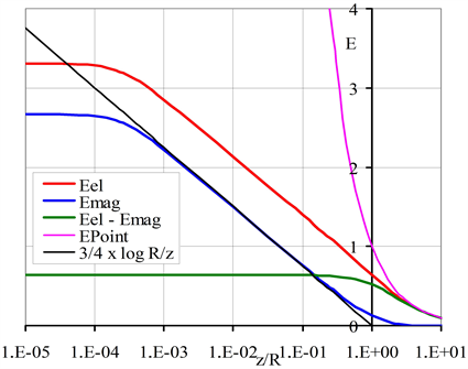
Diagram 2. Related energies $E/m_0{c}^2$ of two real particles as a function of their relative distance $z/R=z/{ƛ}_C$ .

In the range $z/R=z/{ƛ}_C>3$ the magnetic energy is negligible, and the electric energy is nearly identical to the energy (magenta curve) of the fictional point-particle model. At $z/R=z/{ƛ}_C=0.3$ the generation of the rotational kinetic energy is practically complete. In the range $z/{ƛ}_C<3$ is the magnetic energy together with the electric energy responsible for the correct energy inventory. Perhaps not important but remarkable is the fact that the magnetic energy over nearly three decades follows exactly (black curve) the function

$\frac{E}{m_0{c}^2}=\frac{3}{4}\cdot \log \frac{{ƛ}_C}{z}$ (8.23)

9. Multiple Particles

The presented theory predicts the existence of multiple particles consisting of k elementary particles. The multi-electron has the charge

$q_k=k\cdot -e$ (9.1)

the inertial mass,

$m_k=k\cdot m_0$ (9.2)

and the inertial mass energy

$E_{0,k}=k\cdot m_0{c}^2$ (9.3)

Their charge/mass ratio is always

$\frac{q_k}{m_k}=\frac{-e}{m_0}$ (9.4)

According to chapter 5 their angular momentum $J_k$ is always

$J_k=k\cdot m_0\left(1+a\right)\cdot \frac{c}{1+a}\cdot \frac{\hslash }{k\cdot m_{0}c}=\hslash$ (9.5)

So, such multiple particles are not easy to detect. By the way, they are no bosons.

As explained in chapter 5, the angular momentum of the electron is $\hslash$ rather than $\hslash /2$ , and it is the same for all values of k.

The radius $R_k$ is

$R_k={ƛ}_{C,k}=\frac{\hslash }{k\cdot m_{0}c}$ (9.6)

This may be a great advantage of multiple electrons when they travel through liquids (electrolytic processes) or through semiconductors because they have a high “mobility factor”

$\frac{q_k}{R_k}=-e\frac{m_{0}c}{\hslash }\cdot k^2$ (9.7)

The creation of multiple particles needs the input of combination energy $E_{comb}$ . It can be calculated from Equation (7.1) in [3] at the special case $r_2=r_1={ƛ}_C$ :

$\frac{E_{el}\left(r_1,0\right)+\frac{1}{{\beta }_{\phi 1}{\beta }_{\phi 2}}{E_{mag}\left(r_1,0\right)|}_{{\beta }_{\phi 1}={\beta }_{\phi 2}=1}}{\alpha m_0{c}^2\frac{{ƛ}_C}{r_1}\frac{q_1}{e}\frac{q_2}{e}}=\frac{2}{\pi }$ (9.8)

According to the findings of chapter 5 it must be corrected to apply for real stable, charged elementary particles. The result is

$E_{comb}=E_{el}+\frac{1}{{\left(1+a\right)}^2}{E}_{mag}=m_0{c}^2\cdot 4a\cdot \frac{q_1}{e}\frac{q_2}{e}$ (9.9)

where according to (3.10)

$a=\frac{\frac{\alpha }{2\pi }}{1+\frac{\alpha }{2\pi }}=1.160062425\times {10}^{-3}$ (9.10)

Examples:

1) Electron:

$\frac{q_1}{e}\frac{q_2}{e}=\frac{1}{4}$ $E_{comb}=m_0{c}^2\cdot a$ (9.11)

2) Twin electron (Cooper pair)

$\frac{q_1}{e}\frac{q_2}{e}=1$ $E_{comb}=m_0{c}^2\cdot 4a$ (9.12)

$E_{total}=2\cdot E_{totalelectron}+E_{comb}=2m_0{c}^2\left(1+a\right)+m_0{c}^2\cdot 4a$ (9.13)

$E_{total}=2m_0{c}^2\left(1+3a\right)$ (9.14)

The magnetic moment of the twin electron is

${\mu }_2=\frac{2e\hslash }{4m_0}={\mu }_B$ (9.15)

with the erroneous “anomaly” $3a$ .

Generally, the multi-electron consisting of k electrons has the total energy

$E_{k,total}=k\cdot m_0{c}^2\left[1+\left(2k-1\right)a\right]$ (9.16)

The energy

$E_{k,comb}=m_0{c}^2\cdot a\left(2k-1\right)$ (9.17)

must be invested to bind k equal particles together. It is represented by the rotational kinetic energy and should no longer be interpreted as “anomaly” of the magnetic moment. The combination energy is no negative binding energy. When multiple particles are subject to thermal or radiation effects, they may easily decay.

Analogously to (4.8) the relative mass velocity ${\beta }_{m,k}=v_{m,k}/c$ is

${\beta }_{m,k}=\frac{v_{m,k}}{c}=\frac{\sqrt{\left(2k-1\right)a_e\cdot \left[2+\left(2k-1\right)a_e\right]}}{1+\left(2k-1\right)a_e}$ (9.18)

Diagram 3 shows the relative mass velocity $v_{m,k}/c$ of multiple electrons as a function of k. Deviating from the theory, where the factor a according to (9.10) is used, the calculation is based on the measured value

$a_e=1.15965218128\times {10}^{-3}$ (9.19)

according to (3.11).

10. Bound Particles, Lamb Energy, Binding Energy

When charged elementary particles are bound together, their radii $R_b$ increase, and consequently their rotational mass velocities $v_m={\beta }_m\cdot c$ decrease. Conservation of the angular momentum requires according to (4.8) for the rotational velocity $v_b={\beta }_{b}c$ of a bound electron or proton

$m_{0}c\left(1+a\right)\frac{{\beta }_b}{\sqrt{1-{\beta }_b^2}}{R}_b=m_{0}c\left(1+a\right)\frac{{\beta }_m}{\sqrt{1-{\beta }_m^2}}{ƛ}_C$ (10.1)

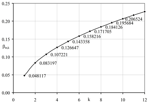
Diagram 3. Mass velocity $v_{m,k}$ of multiple electrons as a function.

From (4.7) and (4.8) follows

$\frac{{\beta }_m}{\sqrt{1-{\beta }_m^2}}=\sqrt{a\left(2+a\right)}$ (10.2)

Thus (10.1) can be reduced to

$\frac{R_b}{{ƛ}_C}=\frac{\sqrt{1-{\beta }_b^2}}{{\beta }_b}\cdot \sqrt{a\left(2+a\right)}$ (10.3)

Finally, ${\beta }_b$ is found to be

${\beta }_b=\frac{\sqrt{a\left(2+a\right)}}{\sqrt{a\left(2+a\right)+{\left(\frac{R_b}{{ƛ}_C}\right)}^2}}=\frac{\sqrt{a\left(2+a\right)}\cdot \frac{{ƛ}_C}{R_b}}{\sqrt{1+a\left(2+a\right){\left(\frac{{ƛ}_C}{R_b}\right)}^2}}$ (10.4)

In hydrogen-like atoms in their ground state is

$R_b=\frac{{ƛ}_C}{\alpha Z}$ (10.5)

and consequently

${\beta }_b=\frac{\sqrt{a\left(2+a\right)}\cdot \alpha Z}{\sqrt{1+a\left(2+a\right)\cdot {\left(\alpha Z\right)}^2}}\approx {\beta }_m\cdot \alpha Z$ (10.6)

Related to excited states ${\beta }_b$ varies according to $\alpha Z/n$ . The total kinetic energy of hydrogen-like atoms, simplified to its non-relativistic form, is

$E_{kin}=\frac{1}{2}{m}_0^{*}{c}^2{\left(\frac{\alpha Z}{n}\right)}^2\left[1+\frac{\alpha Z}{n}\cdot {\beta }_b\right]$ (10.7)

where

$m_0^{*}=\frac{m_0}{1+m_0/m_p}$ (10.8)

is the well-known reduced mass.

${E^{\prime }}_L=\frac{1}{2}{m}_0^{*}{c}^2{\left(\frac{\alpha Z}{n}\right)}^3\cdot {\beta }_b=\frac{1}{2}{m}_0^{*}{c}^2\frac{{\left(\alpha Z\right)}^4}{n^3}$ (10.9)

is the essential part of the Lamb energy.

Besides the kinetic rotational mass velocity $v_m={\beta }_m\cdot c$ the rotational mass energy $m_0{c}^2\cdot a$ contributes to the potential energy and the kinetic energy as well:

When in the equation

$E_{kin}=m_0{c}^2\left(\frac{1}{\sqrt{1-{\beta }^2}}-1\right)$ (10.10)

${\beta }_b$ according to (10.4) is inserted, over

$1-{\beta }_b^2=\frac{1}{1+a\left(2+a\right)\cdot {\frac{{ƛ}_C}{R_b}}^2}$ (10.11)

the result is

$E_{kin}=m_0{c}^2\left[\sqrt{1+a\left(2+a\right)\cdot {\left(\frac{{ƛ}_C}{R_b}\right)}^2}-1\right]\approx a{\left(\frac{{ƛ}_C}{R_b}\right)}^2$ (10.12)

$\frac{E_{kin}}{m_0^{*}{c}^2}=\sqrt{1+a\left(2+a\right)\cdot {\left(\frac{{ƛ}_C}{R_b}\right)}^2}-1\approx a\cdot {\left(\frac{{ƛ}_C}{R_b}\right)}^2$ (10.12a)

where

$R_b=\frac{\alpha Z}{n^2}$ (10.13)

The potential energy (non-relativistic version!) of the hydrogen-like atom including the contribution from the rotational kinetic energy of the electron is then

$\frac{E_{pot}}{m_0^{*}{c}^2}={\left(\frac{\alpha Z}{n}\right)}^2\left[1+a{\left(\frac{{ƛ}_C}{R_n}\right)}^2\right]={\left(\frac{\alpha Z}{n}\right)}^2+\frac{a}{n^2}{\left(\frac{\alpha Z}{n}\right)}^4$ (10.14)

The same effect occurs with the kinetic energy of the hydrogen-like atom, but only at half this value. The ionization energy of the atom is

$E_{ion}=E_{pot}-E_{kin}$ (10.15)

when both the effects resulting from ${\beta }_m$ and a are considered, the total ionization energy becomes

$E_{ion}=\frac{1}{2}{m}_0^{*}{c}^2{\left(\frac{\alpha Z}{n}\right)}^2\left[1-\left(n{\beta }_m-\frac{a}{n^2}\right){\left(\frac{\alpha Z}{n}\right)}^2\right]$ (10.16)

and the Lamb energy is

$E_{Lamb}=\frac{1}{2}{m}_0^{*}{c}^2{\left(\frac{\alpha Z}{n}\right)}^4\left(n{\beta }_m-\frac{a}{n^2}\right)$ (10.17)

The calculation so far is concentrated on the two components of the Lamb energy and disregards relativistic corrections. In Dirac’s well-known equation

$E_{n,j}=\frac{1}{2}\frac{m{c}^2}{1+m/m_p}{\left(\frac{\alpha Z}{n}\right)}^2\left[1+{\left(\frac{\alpha Z}{n}\right)}^2\left(\frac{n}{j+1/2}-\frac{3}{4}\right)\right]$ (10.18)

the Lamb energy is missing. The influence of the Lamb energy is strongest on the s 1/2 levels ( $j=1/2$ ) of the hydrogen atom. The Dirac formula, specialized on $j=1/2$ and completed by the Lamb energy is

$E_{n,j}=\frac{1}{2}\frac{m{c}^2}{1+m/m_p}{\left(\frac{\alpha Z}{n}\right)}^2\left[1+{\left(\frac{\alpha Z}{n}\right)}^2\left(n-\frac{3}{4}-n{\beta }_m+\frac{a}{n^2}\right)\right]$ (10.19)

Table 1 compares the calculated values with and without the Lamb corrections of the presented theory with experimental data.

The accuracy of (10.19) is limited at high values of Z, because it takes only the 2^nd order of the relativistic formula

Table 1. The influence of the lamb energy on the s 1/2 levels of the hydrogen atom.

$E_{ion}=m_0^{*}{c}^2\left(1-\sqrt{1-{\left(\frac{\alpha Z}{n}\right)}^2}\right)$ (10.20)

into account. The respective approximation is

$E_{ion}\approx \frac{1}{2}{m}_0^{*}{c}^2{\left(\frac{\alpha Z}{n}\right)}^2\left[1+\frac{1}{4}{\left(\frac{\alpha Z}{n}\right)}^2\right]$ (10.21)

For comparison Dirac’s formula (10.18) can be written as

$E_{n,j}=\frac{1}{2}{m}_0^{*}{c}^2{\left(\frac{\alpha Z}{n}\right)}^2\left[1+\frac{1}{4}{\left(\frac{\alpha Z}{n}\right)}^2+{\left(\frac{\alpha Z}{n}\right)}^2\left(\frac{n}{j+1/2}-1\right)\right]$ (10.22)

when it is generalized according to (10.20) it becomes

$E_{ion}=m_0^{*}{c}^2\left(1-\sqrt{1-{\left(\frac{\alpha Z}{n}\right)}^2}\right)\left[1+{\left(\frac{\alpha Z}{n}\right)}^2\left(\frac{n}{j+1/2}-1\right)\right]$ (10.23)

To make it complete the relativistic Lamb energy

$E_{Lamb}=m_0^{*}{c}^2\frac{{\left(\frac{\alpha Z}{n}\right)}^2}{\sqrt{1-{\left(\frac{\alpha Z}{n}\right)}^2}}\cdot {\left(\frac{\alpha Z}{n}\right)}^2\cdot \left(n{\beta }_m-\frac{a}{n^2}\right)$ (10.24)

must be subtracted. This is the calculation. But the experimental binding energies of the hydrogen-like atoms, reported at the NIST Atomic Spectra Database Ionization Energies Form, are noticeably different from the calculated results according to (10.23), specialized to $j=1/2$ , and (10.24). The calculated results according to (10.24) are not satisfactory. Better results are achieved when the Lamb energy equation is empirically corrected to

$E_{Lamb}=m_0^{*}{c}^2\frac{{\left(\frac{\alpha Z}{n}\right)}^2}{\sqrt{1-{\left(\frac{\alpha Z}{n}\right)}^2}}\cdot {\left(\frac{\alpha Z}{n}\right)}^2\cdot \left(\frac{n}{\sqrt{Z}}{\beta }_m-\frac{a}{n^2}\right)$ (10.25)

The generally accepted and convenient scale factor ${\left(\alpha Z\right)}^4/n^3$ is not tenable und substituted by the ugly factor ${\left(\alpha Z\right)}^{7/2}/n^3$ , but its efficiency is impressive. Diagram 4 shows the situation.

The non-relativistic approximation (magenta curve) according to (10.16) is not competitive at all. The relativistic calculation according to (10.23), where the non-realistic Lamb energy according to (10.24) is left out (blue curve), shows significant deviations already at small values of Z. When the Lamb energy according to (10.25) is subtracted the result is convincing. In the range $1\le Z\le 70$ the relative deviations of the calculated binding energies from the experimental values are<10⁻⁴. The explanation for this surprising discovery is probably the fact, that the nuclei of hydrogen-like atoms with $Z>1$ are not just charged protons, they contain neutrons with completely unknown influence on the binding energies.

Diagram 5 shows the calculated Lamb energies of hydrogen-like atoms in the Range of $1\le Z\le 100$ according to (10.24).

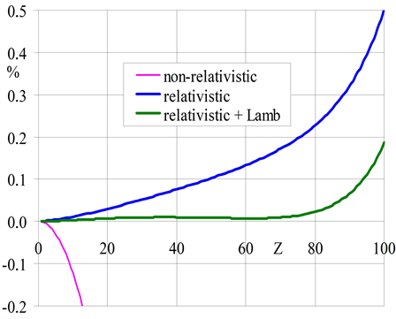
Diagram 4. Relative deviation of calculated binding energies of hydrogen-like atoms from experimental values in the range of $1\le Z\le 100$ .

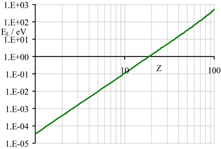
Diagram 5. Calculated lamb energies of hydrogen-like atoms in the range of $1\le Z\le 100$ .

For comparison the author found a typical QED calculation on the Lamb shift [8] . The extensive calculation was introduced—citation: “The Iamb shift includes radiative corrections, corrections due to finite nuclear size, relativistic recoil corrections, and reduced mass corrections of the radiative corrections. We list the individual contributions to the Iamb shift in Table II. These contributions are expressed in terms of a dimensionless, slowly varying function $F\left(Z\alpha \right)$ defined in terms of the level shift $\Delta E$ by the relation

${\Delta }_{LS}E=\frac{\alpha }{\pi }\frac{{\left(Z\alpha \right)}^4}{n^3}\cdot F\left(Z\alpha \right)\cdot m_0{c}^2$ (10.26)

We describe below how each contribution to $F\left(Z\alpha \right)$ which is listed in Table II was determined.

11. Planck Mass, and Gravitational Constant

There is strong evidence that the creation of an electron and a positron from a photon has an impact on spacetime. Mills has given two remarkable equations in his forward-looking book “The Grand Unified Theory of Classical Physics” [9] :

$m_0{c}^2=\cdots =\frac{\alpha h}{1\sec }\sqrt{\frac{{ƛ}_C{c}^2}{2G{m}_0}}$ (Mills Eq. 32.48 b)

$1\sec =\frac{4\pi {\epsilon }_0{ƛ}_C^2{\alpha }^{2}2\pi c}{e^2}\sqrt{\frac{\hslash c}{2G}}{\left(1+\frac{2\pi {\alpha }^2}{2}\right)}^{-2}=0.9975\text{second}$ (Mills Eq. 32.1.2)

Mills’ Eq. 32.48 b is not explicitly derived, but it turns out to be essentially correct. As to Mills’ Eq. 32.1.12, there is no reason why there might be a difference between the space time second “sec” and the MKS second. The key for the right understanding is given by the fact that the total mass $m_{total}$ of the electron is $m_{total}=m_0\left(1+a_e\right)$ rather than the rest mass $m_0$ and that the total energy is $E_{total}=m_0{c}^2\left(1+a_e\right)$ rather than the inertial energy $E_0=m_0{c}^2$ . When Mills developed his theory on “Creation of Matter from Energy” and on “Pair Production” he was confronted with the surprise that the well-established and generally accepted formula

$E_0=hf=m_0{c}^2$ (11.1)

could not be right. Mills’ theory correctly predicts that the creation of matter from energy needs more energy than $E_0=m_0{c}^2$ . Without knowing the total energy and total mass he found no other way out than to suppose, that the spacetime second (“sec”) should be shorter than the MKS second. Thus, he could achieve that the photon energy would be increased from $E_0=m_0{c}^2$ up to the proper value $E_{total}=hf\left(1+a_e\right)$ for the creation of an equivalent particle of a pair. But the accuracy of the result of Eq. (32.1.2) is limited by the accuracy of the measured Gravitational constant G. To come to the correct result, at first Mills’ Eq.32.48 is modified as follows

$m_0{c}^2=\frac{\alpha h}{1\sec }\sqrt{\frac{\hslash c}{2G{m}_0^2}}=\frac{\alpha h}{1\sec }\frac{1}{\sqrt{2}}\cdot \frac{m_{Pl}}{m_0}$ (11.2)

where the definitions of the Compton radius ${ƛ}_C$

${ƛ}_C=\frac{\hslash }{m_{0}c}$ (11.3)

and of the Planck mass

$m_{Pl}=\sqrt{\frac{\hslash c}{G}}$ (11.4)

are used. Now in (11.2) the inertial mass $m_0$ is corrected to $m_{total}=m_0\left(1+a_e\right)$ , and the spacetime second “sec” is corrected to

$1\sec =1\text{MKS-second}=1\text{s}$ (11.5)

Thus, the Planck mass $m_{Pl}$ can be calculated without using the gravitational constant G:

$m_{Pl}=m_e\cdot m_e{c}^2\frac{1\text{s}}{\alpha h}{\left(1+a_e\right)}^2$ (11.6)

when the values of the physical constants according to CODATA 2018 are used, the theoretical value of Planck’s constant becomes

$m_{Plth}=2.176237845\times {10}^{-8}\text{kg}$ $7.5\times {10}^{-10}$ (11.7)

The respective value based on measurements according to CODATA 2018 is

$m_{Pl}=2.17643\times {10}^{-8}\text{kg}$ $1.1\times {10}^{-5}$ (11.8)

From (11.4) and (11.7) follows the theoretical value of the gravitational constant

$G_{th}=\frac{\hslash c}{m_{Pl}^2}=6.675505332\times {10}^{-11}{\text{m}}^3\cdot {\text{kg}}^{-1}\cdot {\text{s}}^{-2}$ $1.5\times {10}^{-9}$ (11.9)

The respective CODATA 2018 value is

$G=6.67430\times {10}^{-11}{\text{m}}^3\cdot {\text{kg}}^{-1}\cdot {\text{s}}^{-2}$ $2.2\times {10}^{-5}$ (11.10)

The important factor

${\left(1+a_e\right)}^{-2}=0.997683906$ $3\times {10}^{-10}$ (11.11)

is known at high precision. If the calculations of $m_{Pl}$ and G are based on the theory constant

$a=\frac{\frac{\alpha }{2\pi }}{1+\frac{\alpha }{2\pi }}=1.160062425\times {10}^{-3}$ $1.5\times {10}^{-10}$ (11.12)

instead of

$a_e=1.15965218128\times {10}^{-3}$ $1.5\times {10}^{-10}$ (11.13)

The gravitational constant G, of course, is slightly different from (11.10):

$G_a=6.675516274\times {10}^{-11}{\text{m}}^3\cdot {\text{kg}}^{-1}\cdot {\text{s}}^{-2}$ $1.5\times {10}^{-9}$ (11.14)

The two theoretical values of G are realistic: The final measured value by BIPM [11] is

$G=6.67554\left(16\right)\times {10}^{-11}{\text{m}}^3\cdot {\text{kg}}^{-1}\cdot {\text{s}}^{-2}$ $2.5\times {10}^{-5}$ (11.15)

Diagram 6 gives a survey of measured values of G since 2000.

The following investigation may help to understand the role of the Planck mass in particle physics. The gravitational energy between two bodies having the masses $m_1$ and $m_2$ at the mutual distance R from their mass center is

$E_G=G\frac{m_1\cdot m_2}{R}$ (11.16)

To separate the two bodies, one of them, for instance $m_2$ , is to be accelerated up to its escape velocity

$v_{esc}={\beta }_{esc}c$ (11.17)

To make the separation complete, the escape velocity must be great enough to reach the radius

$R\to \infty$ (11.18)

The gravitational energy is then totally consumed. The necessary kinetic energy is

$E_{kin}=m_2{c}^2\left(\frac{1}{\sqrt{1-{\beta }_{esc}^2}}-1\right)$ (11.19)

The respective energy condition is

$m_2{c}^2\left(\frac{1}{\sqrt{1-{\beta }_{esc}^2}}-1\right)=G\frac{m_1\cdot m_2}{R}$ (11.20)

Mills [9] applies this principle on an electron/positron pair at identical position and radius

$R={ƛ}_C=\frac{\hslash }{m_{0}c}$ . (11.21)

His calculation is non-relativistic, and his specialized condition is

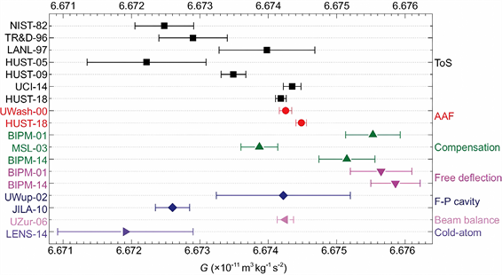
Diagram 6. Survey of measured value of G according to [10] .

$m_1=m_2=m_0$ (11.22)

But the rotational kinetic energy must be taken into account. Before the separation it is $a\cdot m_0{c}^2$ , after the separation it is zero. The correct mass condition is

$m_1=m_2=m_{total}=m_0\left(1+a\right)$ (11.23)

From (11.16), (11.21), and (11.23) follows

$E_G=G\cdot m_0^2{\left(1+a\right)}^2\cdot \frac{m_{0}c}{\hslash }=\frac{G}{\hslash c}\cdot m_0^2{\left(1+a\right)}^2\cdot m_0{c}^2$ (11.24)

with the definition of the Planck Mass according to (11.4) the gravitational energy is

$E_G={\left[\frac{m_0}{m_{Pl}}\cdot \left(1+a\right)\right]}^2\cdot m_0{c}^2={\kappa }^2\cdot m_0{c}^2$ (11.25)

By means of (11.20) the escape velocity according to (11.17) can be calculated:

$\frac{1}{\sqrt{1-{\beta }_{esc}^2}}-1={\left[\frac{m_0}{m_{Pl}}\cdot \left(1+a\right)\right]}^2={\kappa }^2$ (11.26)

$2{\kappa }^2+{\kappa }^4={\left(1+\kappa \right)}^2{\beta }_{esc}^2$ (11.27)

${\beta }_{esc}=\frac{v_{esc}}{c}=\frac{\sqrt{{\kappa }^2\left(2+{\kappa }^2\right)}}{1+{\kappa }^2}$ (11.28)

with the abbreviation

$\kappa =\frac{m_0}{m_{Pl}}\left(1+a\right)$ (11.29)

${\beta }_{esc}=\kappa \sqrt{2}\cdot \frac{\sqrt{1+{\kappa }^2/2}}{1+{\kappa }^2}\approx \kappa \sqrt{2}$ as $\kappa \ll 1$ (11.30)

The factor $\sqrt{2}$ in (11.2) results from the simplified non-relativistic calculation and may lead to wrong interpretations.

${\beta }_{esc}=\frac{\sqrt{3}}{2}=\text{0}\text{.866025}\cdots$ as $\kappa =1$ (11.31)

Diagram 7 demonstrates that the Planck mass is more than just a nice definition. The Planck mass separates weakly relativistic cases from strongly relativistic cases where the escape velocity approaches the velocity of light.

The escape velocity of the electron is

$v_{esc,e}\approx 1.775\times {10}^{-14}\text{m}/\text{s}$ (11.32)

The electric and gravitational forces between to particles are

$F_{el}=\frac{e^2}{4\pi {\epsilon }_0}\cdot \frac{1}{r^2}=\frac{\alpha \hslash c}{r^2}$ (11.33)

and

$F_{gr}=G\cdot \frac{m_0^2}{r^2}$ (11.34)

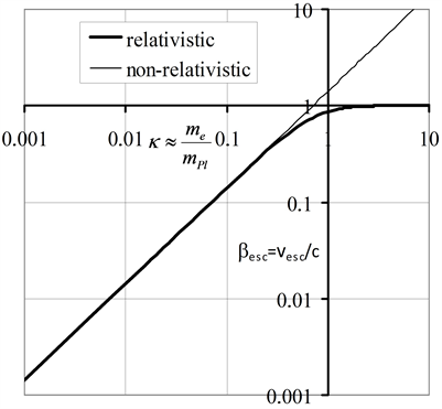
Diagram 7. Relative escape velocity ${\beta }_e=v_e/c$ as a function of the relative mass $m_0/m_{Pl}$ .

The ratio

$\frac{F_{gr}}{F_{el}}=\frac{G}{\alpha \hslash c}\cdot m_0^2$ (11.35)

When the Planck mass according to (11.4) is used the result can be written as

$\frac{F_{gr}}{F_{el}}={\alpha }^{-1}{\left(\frac{m_0}{m_{Pl}}\right)}^2$ (11.36)

Theoretically gravitation affects the internal structure of charged elementary particles, but with the proton the effect is ≈8.1 × 10⁻³⁷ and with the electron only 2.4 × 10⁻⁴³.

12. Results and Conclusions

The circular current loop is a highly efficient and consistent model of the four stable charged particles, namely electron, proton, positron, and antiproton. It is obviously the simplest constituent that perfectly creates their electric and magnetic fields and allows to calculate all physical properties at high accuracy. As the electric and the magnetic fields are unlimited, the radius is the only rational way to define the size of the respective particle. This radius is simply the Compton radius. The calculation of the electric and magnetic properties is demanding, but very productive. Diagram 8 gives a survey of achieved results.

In the range $0.3<z/R=z/{ƛ}_C>3$ the essential part of the rotational kinetic energy is created.

The constant $a=\frac{\alpha }{2\pi }/\left(1+\frac{\alpha }{2\pi }\right)\approx 1.160062\times {10}^{-3}$ is crucial for the presented

theory and has universal importance. It is very close to the “anomaly”

$a_e\approx 1.159652\times {10}^{-3}$ of the magnetic moment of the electron. It could be shown

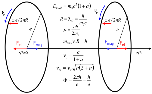
Diagram 8. Survey of calculated basic results, demonstrated at two equal charged elementary particles at a distance of $\approx 2{ƛ}_C$ .

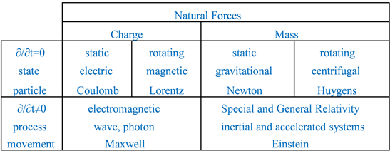
Diagram 9. Survey of proposed four natural forces.

that the magnetic moment of the four stable charged particles is not anomalous but quite regular. This follows from the discovery that the annular particle mass rotates at a specific velocity and thus causes a rotational kinetic energy $E_{rot}=a\cdot m_0{c}^2$ . It completes Einstein’s rest energy $E_0=m_0{c}^2$ and accordingly corrects Planck’s constant. It is the origin of the Lamb shift and enables to calculate the binding energies of the hydrogen-like atoms at high accuracy. The calculation of the axial electric and magnetic forces give rise to the statement that the weak and strong nuclear forces are redundant inventions. There are only three basic natural forces remaining: the electric, the magnetic, and the gravitational forces. The centrifugal force arising from the rotation of the annular particle mass is obviously an additional natural force. A consequence of the disastrous point particle philosophy is the total inability of Quantum-electrodynamics (QED) to handle magnetism in a proper way and results in such nonsensical inventions as the two “intrinsic” nuclear interactions—Consa’s publication [12] on “the state of QED” is very insightful—What really interacts are the classical axial electric and magnetic forces. The Grand Unified Theory (GUT) can no longer be conceived as a problem. Even a theory including all (four?) natural forces is more realistic than ever. The problem is to integrate gravity. The discovery of the rotational kinetic energy is the missing link that allows for the first time to calculate the correct Planck mass and the correct gravitational constant from the electron mass and a few additional fundamental physical constants.

The flat shape of the circular current loop, where the axial dimension is completely missing, removes the perception, electron or proton might have a spherical shape, perhaps like a soap bubble or a massive globe. Needed is only an “equator”. All the rest is not only unnecessary but severely obstructive. The electric and magnetic interactions between two coaxial current loops are significant and important at a distance smaller than twice their radius. That’s the point where the radii of two respective bubbles or globes would get contact and stop the further approach. As electron and proton consist of a flat circular current loop each, the hydrogen atom, too, is a flat object. The neutron, consisting of a proton and an electron, is also supposed to be flat. As a matter of symmetry, the nucleus of Deuterium, too, shouldn’t have an axial dimension. In the physics of subatomic particles and atoms the natural coordinate system is cylindrical rather than spherical. The nucleus of a complex atom should be considered as an object like a skewer, where a series of protons is lined up on a pike and separated from each other by at least one neutron.

The investigation shows that there are indeed four natural forces. But they are significantly different from the present assessment and summarized in Diagram 9.

Conflicts of Interest

This publication was not supported by any university, scientific institute, scientific organization, commercial organization, or private person. There was no scientific, financial, logistic, or administrative support by anyone. I am exclusively driven by personal curiosity and interest.

References

[1]	Bergman, D.L. and Wesley, J.P. (1990) Spinning Charged Ring Model of Electron Yielding Anomalous Magnetic Moment. Galilean Electrodynamics, 1, 63-67.
[2]	Consa, O. (2018) Helical Solenoid Model of the Electron. Progress in Physics, 14, 80-89.
[3]	Landvogt, I.G. (2023) The Circular Current Loop as a Model of Fundamental Particles. https://vixra.org/abs/2308.0188
[4]	Parson, A.L. (1915) A Magneton Theory of the Structure of the Atom. Smithsonian Miscellaneous Collections, 65, 1-80.
[5]	Fundamental Physical Constants, 2018 CODATA Adjustment. http://physics.nist.gov/constants
[6]	van der Togt, C. (2006) The Equivalence of Magnetic and Kinetic Energy. Galilean Electrodynamics, 17, 110-114.
[7]	Comparison of Weak to Strong Interaction. http://hyperphysics.phy-astr.gsu.edu/hbase/Particles/weastr.html
[8]	Johnson, W.R. and Soff, G. (1985) The Lamb Shift in Hydrogen-Like Atoms, . Atomic Data and Nuclear Data Tables, 33, 405-446. https://doi.org/10.1016/0092-640X(85)90010-5
[9]	Mills, R.L. (2020) The Grand Unified Theory of Classical Physics. https://brilliantlightpower.com/book-download-and-streaming/
[10]	Xue, C., et al. (2020) Precision Measurement of the Newtonian Gravitational Constant. National Science Review, 7, 1803-1817. https://doi.org/10.1093/nsr/nwaa165
[11]	Quinn, T., Speake, C., Parks, H. and Davis, R. (2014) The BIPM Measurements of the Newtonian Constant of Gravitation, G. Philosophical Transactions of the Royal Society A: Mathematical, Physical and Engineering Sciences, 372, Article ID: 20140032. https://doi.org/10.1098/rsta.2014.0032
[12]	Consa, O. (2021) Something Is Wrong in the State of QED. ArXiv: 2110.02078.