Second-Order MaxEnt Predictive Modelling Methodology. II: Probabilistically Incorporated Computational Model (2nd-BERRU-PMP)

Dan Gabriel Cacuci

Center for Nuclear Science and Energy, Department of Mechanical Engineering, University of South Carolina, Columbia, SC, USA.

DOI: 10.4236/ajcm.2023.132014                

Abstract

This work presents a comprehensive second-order predictive modeling (PM) methodology based on the maximum entropy (MaxEnt) principle for obtaining best-estimate mean values and correlations for model responses and parameters. This methodology is designated by the acronym 2^nd-BERRU-PMP, where the attribute “2^nd” indicates that this methodology incorporates second- order uncertainties (means and covariances) and second (and higher) order sensitivities of computed model responses to model parameters. The acronym BERRU stands for “Best-Estimate Results with Reduced Uncertainties” and the last letter (“P”) in the acronym indicates “probabilistic,” referring to the MaxEnt probabilistic inclusion of the computational model responses. This is in contradistinction to the 2^nd-BERRU-PMD methodology, which deterministically combines the computed model responses with the experimental information, as presented in the accompanying work (Part I). Although both the 2^nd-BERRU-PMP and the 2^nd-BERRU-PMD methodologies yield expressions that include second (and higher) order sensitivities of responses to model parameters, the respective expressions for the predicted responses, for the calibrated predicted parameters and for their predicted uncertainties (covariances), are not identical to each other. Nevertheless, the results predicted by both the 2^nd-BERRU-PMP and the 2^nd-BERRU-PMD methodologies encompass, as particular cases, the results produced by the extant data assimilation and data adjustment procedures, which rely on the minimization, in a least-square sense, of a user-defined functional meant to represent the discrepancies between measured and computed model responses.

Keywords

Second-Order Predictive Modeling, Data Assimilation, Data Adjustment, Uncertainty Quantification, Reduced Predicted Uncertainties

1. Introduction

An accompanying work [1] has presented a comprehensive second-order predictive modeling (PM) methodology based on the maximum entropy (MaxEnt) principle [2] , for obtaining best-estimate mean values and correlations for model responses and parameters, which was designated by the acronym 2^nd-BERRU-PMD. The attribute “2^nd” indicates that this methodology incorporates second-order uncertainties (means and covariances) and second-order sensitivities of computed model responses to model parameters. The acronym BERRU stands for “Best-Estimate Results with Reduced Uncertainties” and the last letter (“D”) in the acronym indicates “deterministic,” referring to the deterministic inclusion of the computational model responses.

Alternative to the 2^nd-BERRU-PMD methodology, this work presents the 2^nd-BERRU-PMP methodology for obtaining best-estimate mean values and correlations for model responses and parameters. The 2^nd-BERRU-PMP methodology is also based on the MaxEnt principle but includes the computational model responses probabilistically-through a MaxEnt representation-in contradistinction to its deterministic inclusion within the 2^nd-BERRU-PMD methodology. This (contra) distinction is indicated the last letter (“P”) in the acronym, which refers to the “probabilistic” inclusion of the computed model responses.

This work is structured as follows: Section 2 presents the second-order MaxEnt probabilistic representation of the computational model. Section 3 presents the “second order predictive modeling methodology with probabilistically included computed responses” (2^nd-BERRU-PMP) methodology. Although both the 2^nd-BERRU-PMP and the 2^nd-BERRU-PMD methodologies yield expressions that include second (and higher) order sensitivities of responses to model parameters, the respective expressions for the predicted responses, calibrated predicted parameters and their predicted uncertainties (covariances) are not identical to each other, although they encompass, as particular cases, the results produced by the extant data assimilation [3] [4] and data adjustment procedures [5] [6] [7] [8] [9] . Comparisons with the results produced by the first-order BERRU-PM methodology [10] [11] [12] are also presented. The advantages of the 2^nd-BERRU-PMP methodology over the results produced by the data assimilation method [3] [4] are presented in Section 5. The discussion presented in Section 6 concludes this work. Illustrative applications of the 2^nd-BERRU-PMP and the 2^nd-BERRU-PMD methodologies to forward and inverse problems are currently in progress.

2. Second-Order MaxEnt Probabilistic Representation of the Computational Model

The modeling of a physical system requires consideration of the following modeling components:

1) A mathematical model comprising linear and/or nonlinear equations that relate the system’s independent variables and parameters to the system’s state (i.e., dependent) variables. In this work, matrices will be denoted using capital bold letters while vectors will be denoted using either capital or lower-case bold letters. The symbol “ $\triangleq$ ” will be used to denote “is defined as” or “is by definition equal to.” Transposition will be indicated by a dagger ( $†$ ) superscript. The equalities in this work are considered to hold in the weak (“distributional”) sense.

2) Nominal values and uncertainties that characterize the model’s parameters.

3) One or several computational results, customarily referred to as model responses (or objective functions, or indices of performance), which are computed using the mathematical model; and

4) External to the model: experimentally measured responses that correspond to the computed responses, with their respective experimentally determined nominal (mean) values and uncertainties (variances, covariances, skewness, kurtosis, etc.). Occasionally, measurements of correlations among the measured responses and the model parameters, as well as externally performed measurements of model parameters (in addition to the information about parameters used in the model-computations) might be available.

The model parameters usually stem from processes that are external to the physical system (and, hence, model) under consideration and their precise values are seldom, if ever, known. The known characteristics of the model parameters may include their nominal (expected/mean) values and, possibly, higher-order moments (i.e., variance/covariances, skewness, kurtosis), which are usually determined from experimental data and/or processes external to the physical system under consideration. Occasionally, just the lower and the upper bounds may be known for some model parameters. Without loss of generality, the model parameters will be considered in this work to be real-valued scalars, and will be denoted as ${\alpha }_1,\cdots ,{\alpha }_{TP}$ , where the quantity “TP” denotes the “total number of model parameters.” Mathematically, these parameters are considered as components of a TP-dimensional vector denoted as $\alpha \triangleq {\left({\alpha }_1,\cdots ,{\alpha }_{TP}\right)}^{†}\in D_{\alpha }\in {ℝ}^{TP}$ , defined over a domain $D_{\alpha }$ , which is included in a TP-dimensional subset of the ${ℝ}^{TP}$ . The components of the TP-dimensional column vector $\alpha \in {ℝ}^{TP}$ are considered to include imprecisely known geometrical parameters that characterize the physical system’s boundaries in the phase-space of the model’s independent variables. The model parameters can be considered to be quasi-random scalar-valued quantities which follow an unknown multivariate distribution denoted as $p_{\alpha }\left(\alpha \right)$ . The mean values which will be called “nominal” values in the context of computational modeling of the model parameters will be denoted as ${\alpha }_i^0$ ; the superscript “0” will be used throughout this work to denote “nominal values.” These nominal values are formally defined as follows:

${\alpha }_i^0\triangleq {\displaystyle \underset{D_{\alpha }}{\int }{\alpha }_i{p}_{\alpha }\left(\alpha \right)}\text{d}\alpha ,i=1,\cdots ,TP.$ (1)

The expected values of the measured parameters will be considered to constitute the components of a “vector of nominal values” denoted as ${\alpha }^0\triangleq {\left[{\alpha }_1^0,\cdots ,{\alpha }_i^0,\cdots ,{\alpha }_{TP}^0\right]}^{†}$ .

The covariance, $\mathrm{cov}\left({\alpha }_i,{\alpha }_j\right)$ , of two model parameters, ${\alpha }_i$ and ${\alpha }_j$ , is defined as follows:

$\mathrm{cov}\left({\alpha }_i,{\alpha }_j\right)\triangleq {\displaystyle \underset{D_{\alpha }}{\int }\left({\alpha }_i-{\alpha }_i^0\right)\left({\alpha }_j-{\alpha }_j^0\right)p_{\alpha }\left(\alpha \right)}\text{d}\alpha ;i,j=1,\cdots ,TP.$ (2)

The covariances $\mathrm{cov}\left({\alpha }_i,{\alpha }_j\right)$ are considered to be the components of the parameter covariance matrix, denoted as $C_{\alpha \alpha }\triangleq {\left[\mathrm{cov}\left({\alpha }_i,{\alpha }_j\right)\right]}_{TP\times TP}$ .

The results computed using a mathematical model are customarily called “model responses” (or “system responses” or “objective functions” or “indices of performance”). Consider that there are a total number of TR such model responses, each of which can be considered to be a component of the “vector of model responses” $r\triangleq {\left(r_1,\cdots ,r_k,\cdots ,r_{TR}\right)}^{†}$ . Each of these model responses is formally a function (implicit and/or explicit) of the model parameters $\alpha$ , i.e., $r_k=r_k\left(\alpha \right);k=1,\cdots ,TR$ . The uncertainties affecting the model parameters $\alpha$ will “propagate” both directly and indirectly, through the model’s dependent variables, to induce uncertainties in the computed responses, which will therefore be denoted as $r_k^c\left(\alpha \right)$ . Each computed response can be formally expanded in a multivariate Taylor-series around the parameters’ mean values. In particular, the fourth-order Taylor-series of a system response, denoted as $r_k\left(\alpha \right)$ , around the expected (or nominal) parameter values ${\alpha }^0$ has the following formal expression:

$\begin{array}{c}{r}_k\left(\alpha \right)=r_k\left({\alpha }^0\right)+{\displaystyle \underset{j_1=1}{\overset{TP}{\sum }}{\left\{\frac{\partial r_k\left(\alpha \right)}{\partial {\alpha }_{j_1}}\right\}}_{{\alpha }^0}\delta {\alpha }_{j_1}}+\frac{1}{2}{\displaystyle \underset{j_1=1}{\overset{TP}{\sum }}{\displaystyle \underset{j_2=1}{\overset{TP}{\sum }}{\left\{\frac{{\partial }^2{r}_k\left(\alpha \right)}{\partial {\alpha }_{j_1}\partial {\alpha }_{j_2}}\right\}}_{{\alpha }^0}}}\delta {\alpha }_{j_1}\delta {\alpha }_{j_2}\\ +\frac{1}{3!}{\displaystyle \underset{j_1=1}{\overset{TP}{\sum }}{\displaystyle \underset{j_2=1}{\overset{TP}{\sum }}{\displaystyle \underset{j_3=1}{\overset{TP}{\sum }}{\left\{\frac{{\partial }^3{r}_k\left(\alpha \right)}{\partial {\alpha }_{j_1}\partial {\alpha }_{j_2}\partial {\alpha }_{j_3}}\right\}}_{{\alpha }^0}}}}\delta {\alpha }_{j_1}\delta {\alpha }_{j_2}\delta {\alpha }_{j_3}\\ +\frac{1}{4!}{\displaystyle \underset{j_1=1}{\overset{TP}{\sum }}{\displaystyle \underset{j_2=1}{\overset{TP}{\sum }}{\displaystyle \underset{j_3=1}{\overset{TP}{\sum }}{\displaystyle \underset{j_4=1}{\overset{TP}{\sum }}{\left\{\frac{{\partial }^4{r}_k\left(\alpha \right)}{\partial {\alpha }_{j_1}\partial {\alpha }_{j_2}\partial {\alpha }_{j_3}\partial {\alpha }_{j_4}}\right\}}_{{\alpha }^0}}}}}\delta {\alpha }_{j_1}\delta {\alpha }_{j_2}\delta {\alpha }_{j_3}\delta {\alpha }_{j_4}+{\epsilon }_k.\end{array}$ (3)

In Equation (3), the quantity $r_k\left({\alpha }^0\right)$ indicates the computed value of the response using the expected/nominal parameter values ${\alpha }^0\triangleq {\left({\alpha }_1^0,\cdots ,{\alpha }_{TP}^0\right)}^{†}$ . The notation ${\left\{\right\}}_{{\alpha }^0}$ indicates that the quantities within the braces are also computed using the expected/nominal parameter values. The quantity ${\epsilon }_k$ in Equation (3) comprises all quantifiable errors in the representation of the computed response as a function of the model parameters, including the truncation errors $O{\left(\delta {\alpha }_j\right)}^5$ of the Taylor-series expansion, possible bias-errors due to incompletely modeled physical phenomena, and possible random errors due to numerical approximations. The radius/domain of convergence of the series in Equation (3) determines the largest values of the parameter variations $\delta {\alpha }_j$ which are admissible before the respective series becomes divergent. In turn, these maximum admissible parameter variations limit, through Equation (3), the largest parameter covariances/standard deviations which can be considered for using the Taylor-expansion for the subsequent purposes of computing moments of the distribution of computed responses.

As is well known, and as indicated by Equation (3), the Taylor-series of a function of TP-variables [e.g., $r_k\left(\alpha \right)$ ] comprises TP 1^st-order derivatives, $TP\left(TP+1\right)/2$ distinct 2^nd-order derivatives, and so on. The computation by conventional methods of the n^th-order functional derivatives (called “sensitivities” in the field of sensitivity analysis) of a response with respect to the TP-parameters (on which it depends) would require at least $O\left(T{P}^n\right)$ large-scale computations. The exponential increase with the order of response sensitivities of the number of large-scale computations needed to determine higher-order sensitivities is the manifestation of the “curse of dimensionality in sensitivity analysis,” by analogy to the expression coined by Bellman [13] to express the difficulty of using “brute-force” grid search when optimizing a function with many input variables. The “nth-order Comprehensive Adjoint Sensitivity Analysis Methodology for Nonlinear Systems” (nth-CASAM-N) conceived by Cacuci [14] and the “nth-order Comprehensive Adjoint Sensitivity Analysis Methodology for Response-Coupled Forward/Adjoint Linear Systems” (nth-CASAM-L) conceived by Cacuci [15] are currently the only methodologies that enable the exact and efficient computation of arbitrarily high-order sensitivities while overcoming the curse of dimensionality.

Uncertainties in the model’s parameters will evidently give rise to uncertainties in the computed model responses $r_k\left(\alpha \right)$ . The computed model responses are considered to be distributed according to an unknown distribution denoted as $p_c\left(r\right)$ . The unknown joint probability distribution of model parameters and responses will be denoted as $p_c\left(\alpha ,r\right)\triangleq p_{\alpha }\left(\alpha \right)p_c\left(r\right)$ . The approximate moments of the unknown distribution of $r_k\left(\alpha \right)$ are obtained by using the so-called “propagation of errors” methodology, which entails the formal integration over $p_c\left(\alpha ,r\right)\triangleq p_{\alpha }\left(\alpha \right)p_c\left(r\right)$ of various expressions involving the truncated Taylor-series expansion of the response provided in Equation (3). This procedure was first used by Tukey [16] . Tukey’s results were generalized to 6^th-order by Cacuci [15] .

The expectation value, $E_c\left(r_k\right)$ , of a computed response $r_k\left(\alpha \right)$ is obtained by integrating formally Equation (3) over $p_c\left(\alpha ,r\right)$ , which yields the following expression:

$\begin{array}{c}{E}_c\left(r_k\right)\triangleq {\displaystyle \int r_k\left(\alpha \right)p_c\left(\alpha ,r\right)\text{d}\alpha \text{d}r}\\ =r_k\left({\alpha }^0\right)+\frac{1}{2}{\displaystyle \underset{j_1=1}{\overset{TP}{\sum }}{\displaystyle \underset{j_2=1}{\overset{TP}{\sum }}{\left\{\frac{{\partial }^2{r}_k\left(\alpha \right)}{\partial {\alpha }_{j_1}\partial {\alpha }_{j_2}}\right\}}_{{\alpha }^0}\mathrm{cov}\left({\alpha }_{j_1},{\alpha }_{j_2}\right)}}\\ +\frac{1}{6}{\displaystyle \underset{j_1=1}{\overset{TP}{\sum }}{\displaystyle \underset{j_2=1}{\overset{TP}{\sum }}{\displaystyle \underset{j_3=1}{\overset{TP}{\sum }}{\left\{\frac{{\partial }^3{r}_k\left(\alpha \right)}{\partial {\alpha }_{j_1}\partial {\alpha }_{j_2}\partial {\alpha }_{j_3}}\right\}}_{{\alpha }^0}}}}{t}_{j_1{j}_2{j}_3}{\sigma }_{j_1}{\sigma }_{j_2}{\sigma }_{j_3}\\ +\frac{1}{24}{\displaystyle \underset{j_1=1}{\overset{TP}{\sum }}{\displaystyle \underset{j_2=1}{\overset{TP}{\sum }}{\displaystyle \underset{j_3=1}{\overset{TP}{\sum }}{\displaystyle \underset{j_4=1}{\overset{TP}{\sum }}{\left\{\frac{{\partial }^4{r}_k\left(\alpha \right)}{\partial {\alpha }_{j_1}\partial {\alpha }_{j_2}\partial {\alpha }_{j_3}\partial {\alpha }_{j_4}}\right\}}_{{\alpha }^0}}}}}{q}_{j_1{j}_2{j}_3{j}_4}{\sigma }_{j_1}{\sigma }_{j_2}{\sigma }_{j_3}{\sigma }_{j_4}\\ +O\left({\sigma }_{j_1}{\sigma }_{j_2}{\sigma }_{j_3}{\sigma }_{j_4}{\sigma }_{j_5}\right).\end{array}$ (4)

The expectation values $E_c\left(r_k\right)$ , $k=1,\cdots ,TR$ , are considered to be the components of a vector defined as follows: $E_c\left(r\right)\triangleq {\left[E_c\left(r_1\right),\cdots ,E_c\left(r_k\right),\cdots ,E_c\left(r_{TR}\right)\right]}^{†}$ .

The expression of the correlation between a computed responses and a parameter variance, which will be denoted as $\text{cor}\left({\alpha }_i,r_k\right)$ , is presented below:

$\begin{array}{l}\text{cor}\left({\alpha }_i,r_k\right)\triangleq {\displaystyle \int \delta {\alpha }_i\left[r_k\left(\alpha \right)-E_c\left(r_k\right)\right]p_c\left(\alpha ,r\right)\text{d}\alpha \text{d}r}\\ ={\displaystyle \underset{j=1}{\overset{TP}{\sum }}{\left\{\frac{\partial r_k\left(\alpha \right)}{\partial {\alpha }_j}\right\}}_{{\alpha }^0}\mathrm{cov}\left({\alpha }_i,{\alpha }_j\right)}+\frac{1}{2}{\displaystyle \underset{j_1=1}{\overset{TP}{\sum }}{\displaystyle \underset{j_2=1}{\overset{TP}{\sum }}{\left\{\frac{{\partial }^2{r}_k\left(\alpha \right)}{\partial {\alpha }_{j_1}\partial {\alpha }_{j_2}}\right\}}_{{\alpha }^0}}}{t}_{i,j_1{j}_2}{\sigma }_i{\sigma }_{j_1}{\sigma }_{j_2}\\ +\frac{1}{6}{\displaystyle \underset{j_1=1}{\overset{TP}{\sum }}{\displaystyle \underset{j_2=1}{\overset{TP}{\sum }}{\displaystyle \underset{j_3=1}{\overset{TP}{\sum }}{\left\{\frac{{\partial }^3{r}_k\left(\alpha \right)}{\partial {\alpha }_{j_1}\partial {\alpha }_{j_2}\partial {\alpha }_{j_3}}\right\}}_{{\alpha }^0}}}}{q}_{i,j_1{j}_2{j}_3}{\sigma }_{j_1}{\sigma }_{j_2}{\sigma }_{j_3}{\sigma }_{j_4}\\ +O\left({\sigma }_{j_1}{\sigma }_{j_2}{\sigma }_{j_3}{\sigma }_{j_4}{\sigma }_{j_5}\right).\end{array}$ (5)

The correlations $\text{cor}\left({\alpha }_i,r_k\right)$ , $i=1,\cdots ,TP$ , $k=1,\cdots ,TR$ , are considered to be the components of a “parameter-response computed correlation matrix” denoted as $C_{\alpha r}^c$ and defined as follows:

$C_{\alpha r}^c\triangleq \left(\begin{array}{ccc}\text{cor}\left({\alpha }_1,r_1\right)& \cdots & \text{cor}\left({\alpha }_1,r_{TR}\right)\\ ⋮& \ddots & ⋮\\ \text{cor}\left({\alpha }_{TP},r_1\right)& \cdots & \text{cor}\left({\alpha }_{TP},r_{TR}\right)\end{array}\right).$ (6)

The expression of the covariance between two responses $r_k$ and $r_{\mathcal{l}}$ , denoted as $\mathrm{cov}\left(r_k,r_{\mathcal{l}}\right)$ , is presented below:

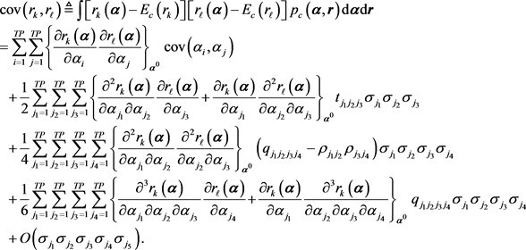(7)

The covariances $\mathrm{cov}\left(r_k,r_{\mathcal{l}}\right)$ , $k,\mathcal{l}=1,\cdots ,TR$ , are considered to be the components of a “computed-responses covariance matrix” denoted as $C_{rr}^c$ and defined as follows:

$C_{rr}^c\triangleq \left(\begin{array}{ccc}\text{cor}\left(r_1,r_1\right)& \cdots & \text{cor}\left(r_1,r_{TR}\right)\\ ⋮& \ddots & ⋮\\ \text{cor}\left(r_{TP},r_1\right)& \cdots & \text{cor}\left(r_{TP},r_{TR}\right)\end{array}\right).$ (8)

The information provided in Equations (1)-(8) regarding the mean values and correlations for the model parameters and computed model responses will be used to construct a second-order MaxEnt approximation, denoted as $p_c\left(z|z_c,C_c\right)$ , to represent the distribution $p_c\left(\alpha ,r\right)\triangleq p_{\alpha }\left(\alpha \right)p_c\left(r\right)$ of computed model responses and parameters. The distribution $p_c\left(z|z_c,C_c\right)$ is constructed by following the procedure outlined in Appendix, to obtain the following expression:

$p_c\left(\alpha ,r\right)\cong p_c\left(z|z_c,C_c\right)\triangleq \frac{{\left(2\pi \right)}^{-\left(TR+TP\right)/2}}{\sqrt{Det\left(C_c\right)}}\exp \left[-\frac{1}{2}{\left(z-z_c\right)}^{†}{C}_c^{-1}\left(z-z_c\right)\right]$ , (9)

where:

$C_c\triangleq \left(\begin{array}{cc}{C}_{rr}^c& C_{r\alpha }^c\\ C_{\alpha r}^c& C_{\alpha \alpha }\end{array}\right);C_{r\alpha }^c\triangleq {\left(C_{\alpha r}^c\right)}^{†};z=\left(\begin{array}{c}r\\ \alpha \end{array}\right);z_c=\left(\begin{array}{c}{E}_c\left(r\right)\\ {\alpha }^0\end{array}\right)$ . (10)

It is important to note that even though the MaxEnt distribution represented in Equation (9) is a multivariate normal distribution characterized by just the first-order moments (mean values) and second-order moments (variance/covariances) of the full but unknown “joint distribution $p_c\left(\alpha ,r\right)$ of computed responses and parameters,” the components of the vector $z_c$ of mean values and the components of the covariance matrix $C_c$ may comprise terms involving third- and higher-order response sensitivities and parameter correlations (e.g., triple and quadruple correlations), if available, as indicated in Equations (4), (5), and (7).

3. 2^nd-BERRU-PMP: Second Order Predictive Modeling Methodology with Probabilistically Included Computed Responses

This Section presents the mathematical and physical considerations leading to the development of the second-order predictive modeling methodology in which the computational model is probabilistically incorporated with the measurements into the combined 2^nd-order MaxEnt posterior distribution which represents all of the available computational and experimental information. This methodology will be designated using the acronym 2^nd-BERRU-PMP, where the last letter (“P”) indicates “probabilistic.” Subsection 3.1 presents the general case, in which measurements (mean values and correlations) for parameters are available−in addition to the information used in the computational model−for incorporation together with the measured responses into the MaxEnt probabilistic representation of the computational model in order to finally obtain the joint posterior distribution that would represent all of the available second-order information. This general case seldom occurs in practice because additional measurements regarding the model parameters (outside of, and in addition to, their use in the model) are rarely available. Usually, only measurements for responses are available for incorporation into the MaxEnt representation of the computational model; this case is analyzed in Subsection 3.2.

3.1. General Case: Measurements for Both Responses and Parameters Are Available for Combination with the MaxEnt Probabilistic Representation of the Computational Model to Obtain Their Joint Posterior Distribution

In the most general case, measurements could be available not only for the responses (results) of interest but also about the parameters used in the model to compute the respective results. In such a case, the second-order MaxEnt distribution which will represent probabilistically the computed model responses and model parameters is to be combined with a second-order MaxEnt distribution which is to represent probabilistically the measured model responses and the additionally measured model parameters (i.e., model parameters measured in addition to, and independently of, the computational model). Since only first- and second-order moments are considered to be available, each of these MaxEnt distributions will be multivariate normal distributions, so their combination will also yield a multivariate posterior MaxEnt distribution (for all of the first- and second-order available moments).

Consider that the total number of experimentally measured responses is TR. The information usually available regarding the distribution of such measured responses comprises the first-order moments (mean values), which will be denoted as $r_i^e$ , $i=1,\cdots ,TR$ , and the second-order moments (variances/covariances), which will be denoted as $\mathrm{cov}{\left(r_i,r_j\right)}_e$ , $i,j=1,\cdots ,TR$ , for the measured responses. Occasionally, measured correlations between the model parameters and the measured responses could also be available. The letter “e” will be used either as a superscript or a superscript to indicate experimentally measured quantities. The expected values of the measured responses will be considered to constitute the components of a vector denoted as $r^e\triangleq {\left(r_1^e,\cdots ,r_{TR}^e\right)}^{†}$ . The covariances of the measured responses are considered to be components of the $TR\times TR$ -dimensional covariance matrix of measured responses, which will be denoted as $C_{rr}^e\triangleq {\left[\mathrm{cov}{\left(r_i,r_j\right)}_e\right]}_{TR\times TR}$ . In principle, it is also possible to obtain correlations between some measured responses and some model parameters. When such correlations between measured responses and measured model parameters are available, they are defined as $\text{cor}{\left({\alpha }_i,r_j\right)}_e$ , $i=1,\cdots ,TP$ ; $j=1,\cdots ,TR$ , and can formally be considered to be elements of a rectangular correlation matrix which will be denoted as $C_{\alpha r}^e\triangleq {\left[\mathrm{cov}{\left({\alpha }_i,r_j\right)}_e\right]}_{TP\times TR}$ . In the most general situation, it is possible to have not only measured responses but also new measurements for the parameters, in addition to and independently of, the parameters used in the mathematical/computational model (i.e., where they are considered to have nominal values ${\alpha }^0$ and covariance matrix $C_{\alpha \alpha }$ ). These measured parameters will be considered to have a vector of mean values denoted as ${\alpha }^e\triangleq \left({\alpha }_1^e,\cdots ,{\alpha }_{TP}^e\right)$ , and a covariance matrix denoted as $C_{\alpha r}^e\triangleq {\left[\mathrm{cov}{\left({\alpha }_i,r_j\right)}_e\right]}_{TP\times TR}$ .

The MaxEnt principle can now be applied, as described in Appendix, to construct the least informative (and hence, most conservative) distribution using the available experimental information, to obtain the following expression:

$p_e\left(z|z_e,C_e\right)=\frac{{\left(2\pi \right)}^{-\left(TR+TP\right)/2}}{\sqrt{Det\left(C_e\right)}}\exp \left[-\frac{1}{2}{\left(z-z_e\right)}^{†}{C}_e^{-1}\left(z-z_e\right)\right],$ (11)

where:

$C_e\triangleq \left(\begin{array}{cc}{C}_{rr}^e& C_{r\alpha }^e\\ C_{\alpha r}^e& C_{\alpha \alpha }^e\end{array}\right);z=\left(\begin{array}{c}r\\ \alpha \end{array}\right);z_e=\left(\begin{array}{c}{r}^e\\ {\alpha }^e\end{array}\right).$ (12)

The joint posterior probability distribution of all computed and experimentally measured quantities, which will be denoted as $p_p\left(z|z_p,C_p\right)$ where the subscript “p” indicates “posterior,” is obtained as the properly normalized product of the distributions $p_e\left(z|z_e,C_e\right)$ and $p_c\left(z|z_c,C_c\right)$ . Since both $p_e\left(z|z_e,C_e\right)$ and $p_c\left(z|z_c,C_c\right)$ are normally distributed, it follows that the posterior probability $p_p\left(z|z_p,C_p\right)$ will also be normally distributed and will be given by the following expression:

$p_p\left(z|z_p,C_p\right)\triangleq p_c\left(z|z_c,C_c\right)p_e\left(z|z_e,C_e\right)=K\exp \left[-\frac{1}{2}Q\left(z|z_p,C_p\right)\right],$ (13)

where the normalization constant K and the quadratic form $Q\left(z_p,C_p\right)$ have the following expressions, respectively:

$K\triangleq {\left(2\pi \right)}^{-N/2}{\left[Det\left(C_c+C_e\right)\right]}^{-1/2}\exp \left[-\frac{1}{2}{\left(z_c-z_e\right)}^{†}{\left(C_c+C_e\right)}^{-1}\left(z_c-z_e\right)\right];$ (14)

$Q\left(z|z_p,C_p\right)\triangleq {\left(z-z_p\right)}^{†}{C}_p^{-1}\left(z-z_p\right);$ (15)

$C_p\triangleq {\left(C_c^{-1}+C_e^{-1}\right)}^{-1}=C_c-C_c{\left(C_c+C_e\right)}^{-1}{C}_c=C_e-C_e{\left(C_c+C_e\right)}^{-1}{C}_e;$ (16)

$z_p\triangleq C_p\left(C_c^{-1}{z}_c+C_e^{-1}{z}_e\right).$ (17)

The expression obtained in Equation (13) provides the exact first-order (mean values) and second-order (variances and co-variances) of the most comprehensive combined distribution of computations and measurements of responses and parameters. In practice, however, such a comprehensive amount of experimental information is highly unlikely to be available. Furthermore, even if such massive amount of experimental information were available, the inversion of the matrix ${\left(C_c+C_e\right)}^{-1}$ may be impractical since it would require massive computational resources when the physical systems involve many (thousands of) parameters.

3.2. Practical Case: Only Response Measurements Are Available for Combination with the MaxEnt Probabilistic Representation of the Computational Model to Obtain Their Joint Posterior Distribution

In practice, the information (mean values and covariances) about the model parameters indicated in Equations (1) and (2) is obtained and assessed prior to using this information in the mathematical/computational model used for computing responses. Thus, all of the information available regarding the model parameters would be used to construct the components of the vector ${\alpha }^0\triangleq {\left({\alpha }_1^0,\cdots ,{\alpha }_{TP}^0\right)}^{†}$ of parameter nominal values and the components of the parameter covariance matrix $C_{\alpha \alpha }$ . In practice, only information about measured responses would become additionally available, i.e., only the vector $r^e\triangleq {\left(r_1^e,\cdots ,r_{TR}^e\right)}^{†}$ and the covariance matrix $C_{rr}^e\triangleq {\left[\mathrm{cov}{\left(r_i,r_j\right)}_e\right]}_{TR\times TR}$ would become available for combination with the computational information. In such a case, the MaxEnt distribution corresponding to Equation (11) will reduce to the following expression:

$p_e\left(r|r^e,C_{rr}^e\right)={\left(2\pi \right)}^{-TR/2}{\left[Det\left(C_{rr}^e\right)\right]}^{-1/2}\exp \left[-\frac{1}{2}{\left(r-r^e\right)}^{†}{\left(C_{rr}^e\right)}^{-1}\left(r-r^e\right)\right].$ (18)

Furthermore, when only the experimental information represented by the distribution $p_e\left(r|r^e,C_{rr}^e\right)$ is available, the posterior joint probability distribution of the computed and measured quantities, which will be denoted as $p_p\left(r,\alpha \right)$ will have the following form:

$\begin{array}{l}{p}_p\left(r,\alpha \right)=N\exp \left[-\frac{1}{2}Q\left(r,\alpha \right)\right];N\triangleq {\left[{\displaystyle \int \exp \left[-\frac{1}{2}Q\left(r,\alpha \right)\right]\text{d}\alpha \text{d}r}\right]}^{-1};\\ Q\left(r,\alpha \right)\triangleq {\left(z-z_c\right)}^{†}{C}_c^{-1}\left(z-z_c\right)+{\left(r-r^e\right)}^{†}{\left(C_{rr}^e\right)}^{-1}\left(r-r^e\right).\end{array}$ (19)

The evaluation of the moments of the posterior distribution represented by Equation (19) will involve the evaluation of ratios of integrals having the following form:

$I={\left[{\displaystyle \int \exp \left[-g\left(z\right)\right]\text{d}z}\right]}^{-1}{\displaystyle \int f\left(z\right)\exp \left[-g\left(z\right)\right]\text{d}z}$ . (20)

The evaluations of expressions such as shown in Equation (20) can be performed to a high degree of accuracy, with a controlled error, by employing the saddle-point (Laplace) method, see e.g., [17] [18] , which yields the following result:

$I=\hat{f}-\frac{1}{2}{\hat{f}}_{i_1}{\hat{g}}_{i_2{i}_3{i}_4}{\hat{g}}^{i_1{i}_2}{\hat{g}}^{i_3{i}_4}+\frac{1}{2}{\hat{f}}_{j_1{j}_2}{\hat{g}}^{j_1{j}_2}+O\left({\hat{f}}_{j_1{j}_2{j}_3}\right)$ , (21)

where:

1) The derivative of a function with respect to a component of $z$ is denoted using a subscript, e.g., $f_i\triangleq \partial f/\partial z_i$ , $f_{ij}\triangleq {\partial }^{2}f/\partial z_i\partial z_j$ , $i,j=1,\cdots ,TI$ , where TI denotes the total number of independent variables;

2) The superscripts denote the respective component of the inverse Hessian of the respective function, e.g., $f^{ij}$ denotes the $\left(i,j\right)$ -element of the inverse Hessian matrix $\left[f_{ij}^{-1}\right]$ ;

3) An index that appears as a subscript and a superscript implies a summation over all possible values of that index;

4) The “hat” denotes that the respective quantity is to be evaluated at the saddle point of $\exp \left[-g\left(z\right)\right]$ , which is defined as the point at which the gradient $g_z\left(z\right)\triangleq \left(\partial g/\partial z_1,\cdots ,\partial g/\partial z_{TI}\right)$ of $g\left(z\right)$ vanishes, i.e., $g_z\left(z\right)=0$ .

The saddle-point of the normalization integral N will be denoted as $\left(r_s,{\alpha }_s\right)$ and is defined by the following relations:

$\frac{\partial Q\left(r,\alpha \right)}{\partial r}=0,\frac{\partial Q\left(r,\alpha \right)}{\partial \alpha }=0,\text{at}\left(r,\alpha \right)=\left(r_s,{\alpha }_s\right).$ (22)

To obtain the partial gradients (differentials) shown in Equation (22), it is convenient to write the matrix $C_c^{-1}$ in the form $C_c^{-1}=\left(\begin{array}{cc}{C}_{11}& C_{12}\\ C_{21}& C_{22}\end{array}\right)$ , and use this form together with the definitions provided in Equations (10) and (12) in Equation (19) to expand the functional $Q\left(r,\alpha \right)$ into the following form:

$\begin{array}{c}Q\left(r,\alpha \right)={\left[r-E_c\left(r\right)\right]}^{†}{C}_{11}\left[r-E_c\left(r\right)\right]+{\left[r-E_c\left(r\right)\right]}^{†}{C}_{12}\left(\alpha -{\alpha }^0\right)\\ +{\left(\alpha -{\alpha }^0\right)}^{†}{C}_{21}\left[r-E_c\left(r\right)\right]+{\left(\alpha -{\alpha }^0\right)}^{†}{C}_{22}\left(\alpha -{\alpha }^0\right)\\ +{\left(r-r^e\right)}^{†}{\left(C_{rr}^e\right)}^{-1}\left(r-r^e\right).\end{array}$ (23)

Taking the partial differentials of the expression in Equation (23) yields the following equation for determining the coordinates of the saddle point $\left(r,\alpha \right)=\left(r_s,{\alpha }_s\right)$ :

$\left(\begin{array}{c}{r}_s-E_c\left(r\right)\\ {\alpha }_s-{\alpha }^0\end{array}\right)=-\left(\begin{array}{cc}{C}_{rr}^c& C_{r\alpha }^c\\ C_{\alpha r}^c& C_{\alpha \alpha }\end{array}\right)\left(\begin{array}{c}{\left(C_{rr}^e\right)}^{-1}\left(r_s-r^e\right)\\ 0\end{array}\right).$ (24)

Solving Equation (24) leads to the following expressions for the coordinates $r_s$ and ${\alpha }_s$ of the saddle point:

$r_s=r^e+C_{rr}^e{\left(C_{rr}^e+C_{rr}^c\right)}^{-1}\left[E_c\left(r\right)-r^e\right]$ , (25)

${\alpha }_s={\alpha }^0-C_{\alpha r}^c{\left(C_{rr}^e+C_{rr}^c\right)}^{-1}\left[E_c\left(r\right)-r^e\right]$ . (26)

The best-estimate predicted mean values for the responses and parameters are defined below:

$r^{bep}\triangleq {\displaystyle \underset{D_p}{\int }r{p}_p\left(\alpha ,r\right)\text{d}\alpha \text{d}r}$ , (27)

${\alpha }^{bep}\triangleq {\displaystyle \underset{D_p}{\int }\alpha p_p\left(\alpha ,r\right)\text{d}\alpha \text{d}r}$ . (28)

The superscript “bep” has been used in Equations (29) and (30), respectively, to indicate that the expressions obtained for the respective predicted responses and parameters are “best estimates with probabilistic computational model.” The saddle-point method is applied to evaluate the integrals represented by Equations (27) and (28), respectively, to obtain the following expressions for the optimally-predicted “best-estimate” values for the responses and calibrated parameters:

$r^{bep}=r_s=r^e+C_{rr}^e{\left(C_{rr}^e+C_{rr}^c\right)}^{-1}\left[E_c\left(r\right)-r^e\right]$ , (29)

${\alpha }^{bep}={\alpha }_s={\alpha }^0-C_{\alpha r}^c{\left(C_{rr}^e+C_{rr}^c\right)}^{-1}\left[E_c\left(r\right)-r^e\right]$ . (30)

Since the components of the vector $E_c\left(r\right)$ , and the components of the matrices $C_{rr}^c$ and $C_{\alpha r}^c$ can contain arbitrarily high-order response sensitivities to model parameters, the expressions presented in Equations (29) and (30) generalize the previous formulas of this type found in data adjustment/assimilation procedures published to date (which contain at most second-order sensitivities). The best-estimate parameter values are the “calibrated model parameters” which can be used for subsequent computations with the “calibrated model.”

The second-order moments of the posterior distribution $p_p\left(r,\alpha \right)$ comprise the covariances between the best estimated response, which will be denoted as $C_{rr}^{bep}$ , the covariances between the best-estimate parameters, which will be denoted as $C_{\alpha \alpha }^{bep}$ , and the correlations between the best-estimate parameters and responses, which will be denoted as $C_{\alpha r}^{bep}$ . The expression of the “best-estimate probabilistic model” posterior parameter covariance matrix, $C_{rr}^{bep}$ , for the best-estimate responses $r^{bep}$ is derived by using the result given in Equation (29) to obtain the following expression:

$C_{rr}^{bep}\triangleq {\displaystyle \underset{D_p}{\int }\left(r-r^{bep}\right){\left(r-r^{bep}\right)}^{†}{p}_p\left(\alpha ,r\right)\text{d}\alpha \text{d}r}=C_{rr}^e-C_{rr}^e{\left(C_{rr}^e+C_{rr}^c\right)}^{-1}{C}_{rr}^e$ . (31)

The following important result has been used to obtain the expression provided in Equation (31):

$\begin{array}{l}\left[E_c\left(r\right)-r^e\right]{\left[E_c\left(r\right)-r^e\right]}^{†}\\ =\left[r-r^e-r+E_c\left(r\right)\right]{\left[r-r^e-r+E_c\left(r\right)\right]}^{†}=C_{rr}^e+C_{rr}^c.\end{array}$ (32)

As indicated in Equation (31), the initial covariance matrix $C_{rr}^e$ for the experimentally measured responses is multiplied by the matrix $\left[I-{\left(C_{rr}^e+C_{rr}^c\right)}^{-1}{C}_{rr}^e\right]$ , which means that the variances contained on the diagonal of the best-estimate matrix $C_{rr}^{bep}$ will be smaller than the experimentally measured variances contained in $C_{rr}^e$ . Hence, the incorporation of experimental information reduces the predicted best-estimate response variances in $C_{rr}^{bep}$ by comparison to the measured variances contained a priori in $C_{rr}^e$ . Since the components of the matrix $C_{rr}^{bep}$ contain high-order sensitivities, the formula presented in Equation (31) generalizes the previous formulas of this type found in data adjustment/assimilation procedures published to date.

The expression of the “best-estimate” posterior parameter covariance matrix $C_{\alpha \alpha }^{bep}$ for the best-estimate parameters ${\alpha }^{bep}$ is derived by using the result given in Equation (30) to obtain:

$C_{\alpha \alpha }^{bep}\triangleq {\displaystyle \underset{D_p}{\int }\left(\alpha -{\alpha }^{bep}\right){\left(\alpha -{\alpha }^{bep}\right)}^{†}{p}_p\left(\alpha ,r\right)\text{d}\alpha \text{d}r}=C_{\alpha \alpha }-C_{\alpha r}^c{\left(C_{rr}^e+C_{rr}^c\right)}^{-1}{C}_{\alpha r}^c.$ (33)

The matrices $C_{\alpha \alpha }$ and $C_{\alpha r}^c{\left(C_{rr}^e+C_{rr}^c\right)}^{-1}{C}_{\alpha r}^c$ are symmetric and positive definite. Therefore, the subtraction indicated in Equation (33) implies that the components of the main diagonal of $C_{\alpha \alpha }^{bep}$ must have smaller values than the corresponding elements of the main diagonal of $C_{\alpha \alpha }$ . In this sense, the combination of computational and experimental information has reduced the best-estimate parameter variances on the diagonal of $C_{\alpha \alpha }^{bep}$ . Since the components of the matrices $C_{\alpha \alpha }$ , $C_{\alpha r}^c$ , and $C_{rr}^c$ contain high-order response sensitivities, the formula presented in Equation (33) generalizes the previous formulas of this type found in data adjustment/assimilation procedures published to date.

The expressions of the “best-estimate” posterior parameter correlation matrix $C_{\alpha r}^{bep}$ and/or its transpose $C_{r\alpha }^{bep}$ , for the best-estimate parameters ${\alpha }^{bep}$ and best-estimate responses $r^{bep}$ , are derived by using the results given in Equation (29) and Equation (30) to obtain the following expressions:

$C_{\alpha r}^{bep}\triangleq {\displaystyle \underset{D_p}{\int }\left(\alpha -{\alpha }^{bep}\right){\left(r-r^{bep}\right)}^{†}{p}_p\left(\alpha ,r\right)\text{d}\alpha \text{d}r}=C_{\alpha r}^e-C_{\alpha r}^c{\left(C_{rr}^e+C_{rr}^c\right)}^{-1}{C}_{rr}^e;$ (34)

$\begin{array}{c}{C}_{r\alpha }^{bep}\triangleq {\displaystyle \underset{D_p}{\int }\left(r-r^{bep}\right){\left(\alpha -{\alpha }^{bep}\right)}^{†}{p}_p\left(\alpha ,r\right)\text{d}\alpha \text{d}r}\\ =C_{r\alpha }^e-C_{rr}^e{\left(C_{rr}^e+C_{rr}^c\right)}^{-1}{C}_{r\alpha }^c={\left(C_{\alpha r}^{bep}\right)}^{†}.\end{array}$ (35)

Since the components of the matrices $C_{\alpha r}^c$ and $C_{rr}^c$ contain high-order sensitivities, the formulas presented in Equations (34) and (35) generalize the previous formulas of this type found in data adjustment/assimilation procedures published to date.

It is important to note from the results shown in Equations (29)-(35) that the computation of the best estimate parameter and response values, together with their corresponding best-estimate covariance matrices, only involves a single matrix inversion when computing ${\left(C_{rr}^e+C_{rr}^c\right)}^{-1}$ , which entails the inversion of a matrix of size $TR\times TR$ . This is computationally very advantageous, since $TR\ll TP$ , i.e., the number of responses is much less than the number of model parameters in the overwhelming majority of practical situations.

Using Equations (24), (29) and (30) in Equation (23) yields the following expression for the minimum value, $Q_{\min }=Q\left({\alpha }^{bep},r^{bep}\right)$ , of the quadratic form $Q\left(\alpha ,r\right)$ :

$\begin{array}{c}{Q}_{\min }={\left(\begin{array}{c}{r}^{bep}-E_c\left(r\right)\\ {\alpha }^{bep}-{\alpha }^0\end{array}\right)}^{†}{\left(\begin{array}{cc}{C}_{rr}^c& C_{r\alpha }^c\\ C_{\alpha r}^c& C_{\alpha \alpha }\end{array}\right)}^{-1}\left(\begin{array}{c}{r}^{bep}-E_c\left(r\right)\\ {\alpha }^{bep}-{\alpha }^0\end{array}\right)\\ +{\left(r^{bep}-r^e\right)}^{†}{\left(C_{rr}^e\right)}^{-1}\left(r^{bep}-r^e\right)\\ ={\left[E_c\left(r\right)-r^e\right]}^{†}{\left(C_{rr}^e+C_{rr}^c\right)}^{-1}\left[E_c\left(r\right)-r^e\right].\end{array}$ (36)

As the expression obtained in Equation (36) indicates, the quantity $Q_{\min }$ represents the square of the length of the vector $\left[E_c\left(r\right)-r^e\right]$ , measuring (in the corresponding metric) the deviations between the experimental and nominally computed responses. The quantity $Q_{\min }$ is independent of calibrating (or adjusting) the original data, so it can be evaluated directly from the given data (i.e., model parameters and computed and measured responses, together with their original uncertainties) after having computed the matrix ${\left(C_{rr}^e+C_{rr}^c\right)}^{-1}$ . As the dimension of the vector $\left[E_c\left(r\right)-r^e\right]$ indicates, the number of degrees of freedom characteristic of the calibration under consideration is equal to the number TR of experimental responses.

4. Inter-Comparison: 2^nd-BERRU-PMP vs. 2^nd-BERRU-PMD

In this section, the results obtained for the best-estimate mean values for the responses and parameters, together with their corresponding best estimate covariances/correlations will be compared to the corresponding results produced by the 2^nd-BERRU-PMD methodology, as well as to the corresponding results produced by the 1^st-BERRU-PM [10] [11] [12] .

4.1. Inter-Comparison of Expressions for the Best-Estimate Predicted Mean Values for Responses

Recall that the 2^nd-BERRU-PMD (best-estimated values with deterministically incorporated computed responses) methodology incorporates deterministically (into the second-order MaxEnt representation of the experimentally measured responses) the following second-order Taylor-expansion of the computed responses:

$\begin{array}{l}r=r^c\left({\alpha }^0\right)+\left[S\left({\alpha }^0\right)\right]\left(\alpha -{\alpha }^0\right)+p\left(\alpha ;{\alpha }^0\right);\\ p\left(\alpha ;{\alpha }^0\right)\triangleq {\left[p_1\left(\alpha ;{\alpha }^0\right),\cdots ,p_{TR}\left(\alpha ;{\alpha }^0\right)\right]}^{†};\\ p_k\left(\alpha ;{\alpha }^0\right)\triangleq \frac{1}{2}{\left(\alpha -{\alpha }^0\right)}^{†}\left[Q_k\left({\alpha }^0\right)\right]\left(\alpha -{\alpha }^0\right).\end{array}$ (37)

In Equation (37), the components of the vector $r^c\left({\alpha }^0\right)\triangleq {\left[r_1^c\left({\alpha }^0\right),\cdots ,r_{TR}^c\left({\alpha }^0\right)\right]}^{†}$ represent the values of the model responses computed at the nominal parameter values ${\alpha }^0$ , and the other vectors and matrices contain first-order and second-order sensitivities of responses with respect to the model parameters, evaluated at the nominal parameter values ${\alpha }^0$ , as defined below:

$\begin{array}{l}S\left(\alpha \right)\triangleq \left(\begin{array}{ccc}{s}_{11}& \cdots & s_{1,TR}\\ ⋮& \ddots & ⋮\\ s_{TR,1}& \cdots & s_{TR,TR}\end{array}\right)\triangleq \left(\begin{array}{ccc}\frac{\partial r_1\left(\alpha \right)}{\partial {\alpha }_1}& \cdots & \frac{\partial r_1\left(\alpha \right)}{\partial {\alpha }_{TP}}\\ ⋮& \ddots & ⋮\\ \frac{\partial r_{TR}\left(\alpha \right)}{\partial {\alpha }_1}& \cdots & \frac{\partial r_{TR}\left(\alpha \right)}{\partial {\alpha }_{TP}}\end{array}\right);\\ Q_k\left(\alpha \right)\triangleq \left(\begin{array}{ccc}{q}_{11}^{\left(k\right)}& \cdots & q_{1,TP}^{\left(k\right)}\\ ⋮& \ddots & ⋮\\ q_{TP,1}^{\left(k\right)}& \cdots & q_{TP,TP}^{\left(k\right)}\end{array}\right)\triangleq \left(\begin{array}{ccc}\frac{{\partial }^2{r}_k^c\left(\alpha \right)}{\partial {\alpha }_1\partial {\alpha }_1}& \cdots & \frac{{\partial }^2{r}_k^c\left(\alpha \right)}{\partial {\alpha }_1\partial {\alpha }_{TP}}\\ ⋮& \ddots & ⋮\\ \frac{{\partial }^2{r}_k^c\left(\alpha \right)}{\partial {\alpha }_{TP}\partial {\alpha }_1}& \cdots & \frac{{\partial }^2{r}_k^c\left(\alpha \right)}{\partial {\alpha }_{TP}\partial {\alpha }_{TP}}\end{array}\right).\end{array}$ (38)

The expressions of the end-results produced the “best-estimated values with deterministically incorporated computed responses” (2^nd-BERRU-PMD) methodology will be designated using the superscript “bed.” The expression obtained using the 2^nd-BERRU-PMD methodology for the best-estimate responses is as follows [1] :

$r^{bed}=r^e+\left(C_{rr}^e-C_{r\alpha }^e{S}^{†}\right){\theta }^{\left(h,n+1\right)}\text{}\text{}\text{}\text{}\text{}\text{}$ , (39)

where the vector ${\theta }^{\left(h,n+1\right)}\triangleq {\left({\theta }_1^{\left(h,n+1\right)},\cdots ,{\theta }_k^{\left(h,n+1\right)},\cdots ,{\theta }_{TR}^{\left(h,n+1\right)}\right)}^{†}$ is the solution of the following iterative (Newton’s method) equation

${\theta }^{\left(n+1\right)}={\theta }^{\left(n\right)}-{\left[A\left({\theta }^{\left(n\right)}\right)\right]}^{-1}w\left({\theta }^{\left(n\right)}\right);\text{}\text{}n=0,1,\cdots .$ (40)

In Equation (40), the components/elements $A_{k,n}\left(\theta \right)$ of the Jacobian matrix $A\left(\theta \right)$ have the following expressions:

$A_{kn}\left(\theta \right)=D_{kn}-V_{kn}\left(\theta \right),$ (41)

where:

$D_{kj}\triangleq {\left(C_{rr}^e+S{C}_{\alpha \alpha }{S}^{†}-C_{r\alpha }^e{S}^{†}-S{C}_{\alpha r}^e\right)}_{kj},D\triangleq {\left[D_{kj}\right]}_{TR\times TR}$ ; (42)

$V_{kn}\left(\theta \right)\triangleq {\displaystyle \underset{j=1}{\overset{TR}{\sum }}{\theta }_j\left[M_{nj}^{\left(k\right)}+M_{kj}^{\left(n\right)}+M_{kn}^{\left(j\right)}\right]},V\left(\theta \right)\triangleq {\left[V_{kn}\left(\theta \right)\right]}_{TR\times TR}.$ (43)

$M^{\left(k\right)}\text{}\triangleq {\left[M_{ij}^{\left(k\right)}\right]}_{TR\times TR}\triangleq {\left(C_{\alpha r}^e-C_{\alpha \alpha }{S}^{†}\right)}^{†}\left[Q_k\left({\alpha }^0\right)\right]\left(C_{\alpha r}^e-C_{\alpha \alpha }{S}^{†}\right)={\left[M^{\left(k\right)}\right]}^{†}$ . (44)

$w\left(\theta \right)\triangleq {\left[w_1\left(\theta \right),\cdots ,w_k\left(\theta \right),\cdots ,w_{TR}\left(\theta \right)\right]}^{†}\triangleq -d+D\theta +u\left(\theta \right)$ . (45)

$d\triangleq r^c\left({\alpha }^0\right)-r^e;\text{}d\triangleq {\left(d_1,\cdots ,d_{TR}\right)}^{†};d_1\triangleq r_i^c\left({\alpha }^0\right)-r_i^e;i=1,\cdots ,TR.$ (46)

$u\left(\theta \right)\triangleq {\left[u_1\left(\theta \right),\cdots ,u_{TR}\left(\theta \right)\right]}^{†};\text{}{u}_k\left(\theta \right)\triangleq -\frac{1}{2}{\theta }^{†}{M}^{\left(k\right)}\theta -{\displaystyle \underset{i=1}{\overset{TR}{\sum }}{\theta }_i}{\displaystyle \underset{j=1}{\overset{TR}{\sum }}{M}_{kj}^{\left(i\right)}{\theta }_j}.$ (47)

The initial iterate for starting the iterations for obtaining solution of Equation (40) can be chosen [1] as follows:

${\theta }^{\left(h,0\right)}\triangleq {\left({\theta }_1^{\left(h,0\right)},\cdots ,{\theta }_j^{\left(h,0\right)},\cdots ,{\theta }_{TR}^{\left(h,0\right)}\right)}^{†};{\theta }_j^{\left(h,0\right)}=2D_{jj}/3M_{jj}^{\left(j\right)};j=1,\cdots ,TR.$ (48)

$A_{kn}\left({\theta }^{\left(h,0\right)}\right)=D_{kn}-{\displaystyle \underset{j=1}{\overset{TR}{\sum }}{\theta }_j^{\left(h,0\right)}\left[M_{nj}^{\left(k\right)}+M_{kj}^{\left(n\right)}+M_{kn}^{\left(j\right)}\right]}.$ (49)

$w_k\left({\theta }^{\left(h,0\right)}\right)=u_k\left({\theta }^{\left(h,0\right)}\right)+{\displaystyle \underset{j=1}{\overset{TR}{\sum }}{D}_{kj}}{\theta }_j^{\left(h,0\right)}-d_k,k=1,\cdots ,TR;$ (50)

$\begin{array}{c}{u}_k\left({\theta }^{\left(h,0\right)}\right)=-\frac{1}{2}{\displaystyle \underset{i=1}{\overset{TR}{\sum }}{\displaystyle \underset{j=1}{\overset{TR}{\sum }}{\theta }_i^{\left(h,0\right)}{M}_{ij}^{\left(k\right)}{\theta }_j^{\left(h,0\right)}}}-{\displaystyle \underset{i=1}{\overset{TR}{\sum }}{\theta }_i^{\left(h,0\right)}}{\displaystyle \underset{j=1}{\overset{TR}{\sum }}{M}_{kj}^{\left(i\right)}{\theta }_j^{\left(h,0\right)}}\\ \cong -\frac{4}{9}{\displaystyle \underset{i=1}{\overset{TR}{\sum }}{\displaystyle \underset{j=1}{\overset{TR}{\sum }}\left(\frac{D_{ii}}{M_{ii}^{\left(i\right)}}\right)\left(\frac{D_{jj}}{M_{jj}^{\left(j\right)}}\right)\left[\frac{1}{2}{M}_{ij}^{\left(k\right)}+M_{kj}^{\left(i\right)}\right]}},k=1,\cdots ,TR.\end{array}$ (51)

The first-iterate ${\theta }^{\left(h,1\right)}$ of the solution of Equation (40) has the following expression:

$\begin{array}{l}{\theta }^{\left(h,1\right)}={\theta }^{\left(h,0\right)}-{\left(D-V^{\left(h,0\right)}\right)}^{-1}\left(u^{\left(h,0\right)}+D{\theta }^{\left(h,0\right)}-d\right);\\ V^{\left(h,0\right)}\triangleq V\left({\theta }^{\left(h,0\right)}\right);u^{\left(h,0\right)}\triangleq u\left({\theta }^{\left(h,0\right)}\right).\end{array}$ (52)

Using the first-iterate, ${\theta }^{\left(h,1\right)}$ , in Equation (39) yields the following expressions for the “first-iterate best-estimate” values for the responses:

$\begin{array}{l}{r}^{\left(1\right)bed}=r^e+r^{(0)};\\ r^{\left(0\right)}\triangleq \left(C_{rr}^e-C_{r\alpha }^e{S}^{†}\right)\left[{\theta }^{\left(h,0\right)}-{\left(D-V^{\left(h,0\right)}\right)}^{-1}\left(u^{\left(h,0\right)}+D{\theta }^{\left(h,0\right)}-d\right)\right].\end{array}$ (53)

It is noteworthy that the “vector of deviations” $d$ can be considered to be a (quasi-) random variable; it has been shown in [1] that the “vector of mean values of deviations” $\bar{d}\triangleq {\left[{\bar{d}}_1,\cdots ,{\bar{d}}_{TR}\right]}^{†}$ and the covariance matrix $D\triangleq {\left[D_{ij}\right]}_{TR\times TR}$ of the vector of deviations $d$ have the following expressions (up to second-order sensitivities):

$\text{}\text{}\text{}\text{}\text{}\text{}\text{}\text{}\bar{d}={\left[Q_1\left({\alpha }^0\right)C_{\alpha \alpha },\cdots ,Q_{TR}\left({\alpha }^0\right)C_{\alpha \alpha }\right]}^{†}$ ; (54)

$D=C_{rr}^e+S{C}_{\alpha \alpha }{S}^{†}-C_{r\alpha }^e{S}^{†}-S{C}_{\alpha r}^e$ . (55)

Comparing the expression of the first-iterate, cf., Equation (53) produced by the 2^nd-BERRU-PMD methodology with the corresponding expression produced by the 2^nd-BERRU-PMP methodology, cf. Equation (29), indicates that both expressions include the second-order sensitivities of the responses with respect to the parameters, but in distinct ways. Furthermore, the expression produced by the 2^nd-BERRU-PMP methodology, cf. Equation (29), can include all of the response sensitivities and parameter correlations of order higher than two, if available. Such an inclusion of higher-order sensitivities and parameter correlations is not provided by the result, cf. Equation (53), obtained using the 2^nd-BERRU-PMD methodology.

The expression provided in Equation (29) coincides with the expression provided in Equation (53) only if the following relationship holds:

$\begin{array}{l}{r}^{bep}=r^{\left(1\right)bed}\text{iff}:C_{rr}^e{\left(C_{rr}^e+C_{rr}^c\right)}^{-1}\left[E_c\left(r\right)-r^e\right]\\ =\left(C_{rr}^e-C_{r\alpha }^e{S}^{†}\right)\left[{\theta }^{\left(h,0\right)}-{\left(D-V^{\left(h,0\right)}\right)}^{-1}\left(u^{\left(h,0\right)}+D{\theta }^{\left(h,0\right)}-d\right)\right].\end{array}$ (56)

The equality in Equation (56) can hold if the following conditions are simultaneously satisfied: $C_{r\alpha }^e=0$ , ${\theta }^{\left(h,0\right)}=0$ , $V^{\left(h,0\right)}=0$ , $u^{\left(h,0\right)}=0$ , $C_{rr}^c=S{C}_{\alpha \alpha }{S}^{†}$ , $d=\left[E_c\left(r\right)-r^e\right]$ , in which case we also have the relation $D=C_{rr}^e+S{C}_{\alpha \alpha }{S}^{†}=C_{rr}^e+C_{rr}^c$ . These conditions are satisfied if all of the sensitivities higher than first-order are ignored, and if the experimental responses are uncorrelated to the model parameters. In this particular case, the results produced by the 2^nd-BERRU-PMP and 2^nd-BERRU-PMD methodologies also coincide with the results produced by the first-order 1^st-BERRU-PM methodology.

4.2. Inter-Comparison of Expressions for the Best-Estimate Predicted Mean Values for Parameters

The expression obtained using the 2^nd-BERRU-PMD methodology for the best-estimate parameters is as follows [1] :

${\alpha }^{bed}={\alpha }^0+\left(C_{\alpha r}^e-C_{\alpha \alpha }{S}^{†}\right){\theta }^{\left(h,n+1\right)}$ . (57)

Using the first-iterate ${\theta }^{\left(h,1\right)}$ in Equation (57) yields the following first-iterate expression for the best-estimate parameters:

$\begin{array}{l}{\alpha }^{\left(1\right)bed}={\alpha }^0+{\beta }^{\left(0\right)};\\ {\beta }^{\left(0\right)}\triangleq \left(C_{\alpha r}^e-C_{\alpha \alpha }{S}^{†}\right)\left[{\theta }^{\left(h,0\right)}-{\left(D-V^{\left(h,0\right)}\right)}^{-1}\left(u^{\left(h,0\right)}+D{\theta }^{\left(h,0\right)}-d\right)\right].\end{array}$ (58)

Comparing the expression provided in Equation (58), namely the first-iterate produced by the 2^nd-BERRU-PMD methodology, with the corresponding expression produced by the 2^nd-BERRU-PMP methodology, cf. Equation (30), indicates that both expressions include the second-order sensitivities of the responses with respect to the parameters, but in distinct ways. Furthermore, the expression produced by the 2^nd-BERRU-PMP methodology, cf. Equation (30), can include all of the response sensitivities and parameter correlations of order higher than two, if available. Such an inclusion of higher-order sensitivities and parameter correlations is not possible with the result obtained using the 2^nd-BERRU-PMD methodology, cf. Equation (58).

The expression provided in Equation (30) coincides with the expression provided in Equation (58) only if the following relationship holds:

$\begin{array}{l}{\alpha }^{bep}={\alpha }^{\left(1\right)bed}\text{iff}:-C_{\alpha r}^c{\left(C_{rr}^e+C_{rr}^c\right)}^{-1}\left[E_c\left(r\right)-r^e\right]\\ =\left(C_{\alpha r}^e-C_{\alpha \alpha }{S}^{†}\right)\left[{\theta }^{\left(h,0\right)}-{\left(D-V^{\left(h,0\right)}\right)}^{-1}\left(u^{\left(h,0\right)}+D{\theta }^{\left(h,0\right)}-d\right)\right].\end{array}$ (59)

The equality in Equation (59) can hold if the following conditions are simultaneously satisfied: $C_{\alpha r}^e=0$ , ${\theta }^{\left(h,0\right)}=0$ , $V^{\left(h,0\right)}=0$ , $u^{\left(h,0\right)}=0$ , $C_{rr}^c=S{C}_{\alpha \alpha }{S}^{†}$ , $d=\left[E_c\left(r\right)-r^e\right]$ , in which case we also have the relation $D=C_{rr}^e+S{C}_{\alpha \alpha }{S}^{†}=C_{rr}^e+C_{rr}^c$ . These conditions are satisfied if all of the sensitivities higher than first-order are ignored. In this particular case, the results produced by the 2^nd-BERRU-PMP and 2^nd-BERRU-PMD methodologies also coincide with the results produced by the first-order 1^st-BERRU-PM methodology.

4.3. Inter-Comparison of Expressions for the Best-Estimate Predicted Response Covariances

The expression obtained using the 2^nd-BERRU-PMD methodology [1] for the “first-iterate best-estimate” covariance matrix $C_{rr}^{\left(1\right)bed}$ for the responses is as follows:

$\begin{array}{c}{C}_{rr}^{\left(1\right)bed}=C_{rr}^e-C_{rd}^{\left(1\right)}{Y}_r^{†}+X_r{\theta }^{\left(h,0\right)}{\left({\theta }^{\left(h,0\right)}\right)}^{†}{X}_r^{†}-X_r{\theta }^{\left(h,0\right)}{\bar{d}}^{†}{Y}_r^{†}\\ +X_r{\theta }^{\left(h,0\right)}{\left(u^{\left(h,0\right)}\right)}^{†}{Y}_r^{†}-Y_r{\left(C_{rd}^{\left(1\right)}\right)}^{†}-Y_r\bar{d}{\left({\theta }^{\left(h,0\right)}\right)}^{†}{X}_r^{†}\\ +Y_{r}D{Y}_r^{†}-Y_r\bar{d}{\left(u^{\left(h,0\right)}\right)}^{†}{Y}_r^{†}+Y_r{u}^{\left(h,0\right)}{\left({\theta }^{\left(h,0\right)}\right)}^{†}{X}_r^{†}\\ -Y_r{u}^{\left(h,0\right)}{\bar{d}}^{†}{Y}_r^{†}+Y_r{u}^{\left(h,0\right)}{\left(u^{\left(h,0\right)}\right)}^{†}{Y}_r^{†}.\end{array}$ (60)

where:

$C_{rd}^{\left(1\right)}=C_{rr}^e-C_{r\alpha }^e{S}^{†};X_r\triangleq C_{rd}^{\left(1\right)}\left[{\left(D-V^{\left(h,0\right)}\right)}^{-1}D-I\right];Y_r\triangleq C_{rd}^{\left(1\right)}{\left(D-V^{\left(h,0\right)}\right)}^{-1}.$ (61)

Comparing the 2^nd-BERRU-PMD-expression provided in Equation (60) with the corresponding expression obtained using the 2^nd-BERRU-PMP methodology, cf. Equation (31), indicates that both expressions include the second-order sensitivities of the responses with respect to the parameters, but in distinct ways. Furthermore, the expression produced by the 2^nd-BERRU-PMP methodology, cf. Equation (31), can include all of the response sensitivities and parameter correlations of order higher than two, if available. Such an inclusion of higher-order sensitivities and parameter correlations is not possible with the result obtained using the 2^nd-BERRU-PMD methodology, cf. Equation (60).

The expression provided in Equation (31) coincides with the expression provided in Equation (60) only if the following relationship holds:

$\begin{array}{l}{C}_{rr}^{bep}=C_{rr}^{\left(1\right)bed}\text{iff}:-C_{rr}^e{\left(C_{rr}^e+C_{rr}^c\right)}^{-1}{C}_{rr}^e=-C_{rd}^{\left(1\right)}{Y}_r^{†}+X_r{\theta }^{\left(h,0\right)}{\left({\theta }^{\left(h,0\right)}\right)}^{†}{X}_r^{†}\\ -X_r{\theta }^{\left(h,0\right)}{\bar{d}}^{†}{Y}_r^{†}+X_r{\theta }^{\left(h,0\right)}{\left(u^{\left(h,0\right)}\right)}^{†}{Y}_r^{†}-Y_r{\left(C_{rd}^{\left(1\right)}\right)}^{†}-Y_r\bar{d}{\left({\theta }^{\left(h,0\right)}\right)}^{†}{X}_r^{†}+Y_{r}D{Y}_r^{†}\\ -Y_r\bar{d}{\left(u^{\left(h,0\right)}\right)}^{†}{Y}_r^{†}+Y_r{u}^{\left(h,0\right)}{\left({\theta }^{\left(h,0\right)}\right)}^{†}{X}_r^{†}-Y_r{u}^{\left(h,0\right)}{\bar{d}}^{†}{Y}_r^{†}+Y_r{u}^{\left(h,0\right)}{\left(u^{\left(h,0\right)}\right)}^{†}{Y}_r^{†}.\end{array}$ (62)

The equality shown in Equation (62) can hold only if all of the second-order sensitivities are neglected, and if the experimental responses are uncorrelated to the model parameters, in which case the following simplifications occur: $X_r=0$ , $Y_r=C_{rd}^{\left(1\right)}{D}^{-1}$ , and $C_{rd}^{\left(1\right)}=C_{rr}^e$ , in which case we also have the relation $D=C_{rr}^e+S{C}_{\alpha \alpha }{S}^{†}=C_{rr}^e+C_{rr}^c$ . In this particular case, the results produced by the 2^nd-BERRU-PMP and 2^nd-BERRU-PMD methodologies also coincide with the results produced by the first-order 1^st-BERRU-PM methodology.

4.4. Inter-Comparison of Expressions for the Best-Estimate Predicted Parameter Covariances

The expression obtained using the 2^nd-BERRU-PMD methodology [1] for the “first-iterate best-estimate” covariance matrix $C_{\alpha \alpha }^{\left(1\right)be}$ for the model parameters is as follows:

$\begin{array}{c}{C}_{\alpha \alpha }^{\left(1\right)bed}=C_{\alpha \alpha }^e-C_{\alpha d}^{\left(1\right)}{Y}_{\alpha }^{†}+X_{\alpha }{\theta }^{\left(h,0\right)}{\left({\theta }^{\left(h,0\right)}\right)}^{†}{X}_{\alpha }^{†}-X_{\alpha }{\theta }^{\left(h,0\right)}{\bar{d}}^{†}{Y}_{\alpha }^{†}\\ +X_{\alpha }{\theta }^{\left(h,0\right)}{\left(u^{\left(h,0\right)}\right)}^{†}{Y}_{\alpha }^{†}-Y_{\alpha }{\left(C_{\alpha d}^{\left(1\right)}\right)}^{†}-Y_{\alpha }\bar{d}{\left({\theta }^{\left(h,0\right)}\right)}^{†}{X}_{\alpha }^{†}\\ +Y_{\alpha }D{Y}_{\alpha }^{†}-Y_{\alpha }\bar{d}{\left(u^{\left(h,0\right)}\right)}^{†}{Y}_{\alpha }^{†}+Y_{\alpha }{u}^{\left(h,0\right)}{\left({\theta }^{\left(h,0\right)}\right)}^{†}{X}_{\alpha }^{†}\\ -Y_{\alpha }{u}^{\left(h,0\right)}{\bar{d}}^{†}{Y}_{\alpha }^{†}+Y_{\alpha }{u}^{\left(h,0\right)}{\left(u^{\left(h,0\right)}\right)}^{†}{Y}_{\alpha }^{†}.\end{array}$ (63)

were:

$C_{\alpha d}^{\left(1\right)}=C_{\alpha r}^e-C_{\alpha \alpha }^e{S}^{†};X_{\alpha }\triangleq C_{\alpha d}^{\left(1\right)}\left[{\left(D-V^{\left(h,0\right)}\right)}^{-1}D-I\right];Y_{\alpha }\triangleq C_{\alpha d}^{\left(1\right)}{\left(D-V^{\left(h,0\right)}\right)}^{-1}.$ (64)

Comparing the 2^nd-BERRU-PMD-expression provided in Equation (63) with the corresponding expression obtained using the 2^nd-BERRU-PMP methodology, cf. Equation (33), indicates that both expressions include the second-order sensitivities of the responses with respect to the parameters, but in distinct ways. Furthermore, the expression produced by the 2^nd-BERRU-PMP methodology, cf. Equation (33), can include all of the response sensitivities and parameter correlations of order higher than two, if available. Such an inclusion of higher-order sensitivities and parameter correlations is not possible with the result obtained using the 2^nd-BERRU-PMD methodology, cf. Equation (63).

The expression provided in Equation (33) coincides with the expression provided in Equation (63) only if the following relationship holds:

$\begin{array}{l}{C}_{\alpha \alpha }^{bep}=C_{\alpha \alpha }^{\left(1\right)bed}\text{iff}:\text{}\text{}\text{}\text{}-C_{\alpha r}^c{\left(C_{rr}^e+C_{rr}^c\right)}^{-1}{C}_{\alpha r}^c=-C_{\alpha d}^{\left(1\right)}{Y}_{\alpha }^{†}+X_{\alpha }{\theta }^{\left(h,0\right)}{\left({\theta }^{\left(h,0\right)}\right)}^{†}{X}_{\alpha }^{†}\\ -X_{\alpha }{\theta }^{\left(h,0\right)}{\bar{d}}^{†}{Y}_{\alpha }^{†}+X_{\alpha }{\theta }^{\left(h,0\right)}{\left(u^{\left(h,0\right)}\right)}^{†}{Y}_{\alpha }^{†}-Y_{\alpha }{\left(C_{\alpha d}^{\left(1\right)}\right)}^{†}-Y_{\alpha }\bar{d}{\left({\theta }^{\left(h,0\right)}\right)}^{†}{X}_{\alpha }^{†}+Y_{\alpha }D{Y}_{\alpha }^{†}\\ -Y_{\alpha }\bar{d}{\left(u^{\left(h,0\right)}\right)}^{†}{Y}_{\alpha }^{†}+Y_{\alpha }{u}^{\left(h,0\right)}{\left({\theta }^{\left(h,0\right)}\right)}^{†}{X}_{\alpha }^{†}-Y_{\alpha }{u}^{\left(h,0\right)}{\bar{d}}^{†}{Y}_{\alpha }^{†}+Y_{\alpha }{u}^{\left(h,0\right)}{\left(u^{\left(h,0\right)}\right)}^{†}{Y}_{\alpha }^{†}.\end{array}$ (65)

The equality shown in Equation (65) can hold only if all of the second-order sensitivities are neglected, and if the experimental responses are uncorrelated to the model parameters, in which case the following simplifications occur: $X_{\alpha }=0$ , $Y_{\alpha }=C_{\alpha d}^{\left(1\right)}{D}^{-1}$ , in which case we also have the relation $D=C_{rr}^e+S{C}_{\alpha \alpha }{S}^{†}=C_{rr}^e+C_{rr}^c$ . In this particular case, the results produced by the 2^nd-BERRU-PMP and 2^nd-BERRU-PMD methodologies also coincide with the results produced by the first-order 1^st-BERRU-PM methodology.

4.5. Inter-Comparison of Expressions for the Best-Estimate Predicted Correlations between Parameters and Responses

The expression obtained using the 2^nd-BERRU-PMD methodology [1] for the “first-iterate best-estimate” correlation matrix $C_{\alpha r}^{\left(1\right)bed}$ for the parameters and responses is as follows:

$\begin{array}{c}{C}_{\alpha r}^{\left(1\right)bed}=C_{\alpha r}^e-C_{\alpha d}^{\left(1\right)}{Y}_r^{†}+X_{\alpha }{\theta }^{\left(h,0\right)}{\left({\theta }^{\left(h,0\right)}\right)}^{†}{X}_r^{†}-X_{\alpha }{\theta }^{\left(h,0\right)}{\bar{d}}^{†}{Y}_r^{†}\\ +X_{\alpha }{\theta }^{\left(h,0\right)}{\left(u^{\left(h,0\right)}\right)}^{†}{Y}_r^{†}-Y_{\alpha }{\left(C_{rd}^{\left(1\right)}\right)}^{†}-Y_{\alpha }\bar{d}{\left({\theta }^{\left(h,0\right)}\right)}^{†}{X}_r^{†}\\ +Y_{\alpha }D{Y}_r^{†}-Y_{\alpha }\bar{d}{\left(u^{\left(h,0\right)}\right)}^{†}{Y}_r^{†}+Y_{\alpha }{u}^{\left(h,0\right)}{\left({\theta }^{\left(h,0\right)}\right)}^{†}{X}_r^{†}\\ -Y_{\alpha }{u}^{\left(h,0\right)}{\bar{d}}^{†}{Y}_r^{†}+Y_{\alpha }{u}^{\left(h,0\right)}{\left(u^{\left(h,0\right)}\right)}^{†}{Y}_r^{†}.\end{array}$ (66)

Comparing the 2^nd-BERRU-PMD-expression provided in Equation (66) with the corresponding expression obtained using the 2^nd-BERRU-PMP methodology, cf. Equation (34), indicates that both expressions include the second-order sensitivities of the responses with respect to the parameters, but in distinct ways. Furthermore, the expression produced by the 2^nd-BERRU-PMP methodology, cf. Equation (34), can include all of the response sensitivities and parameter correlations of order higher than two, if available. Such an inclusion of higher-order sensitivities and parameter correlations is not possible with the result obtained using the 2^nd-BERRU-PMD methodology, cf. Equation (66)

The expression provided in Equation (34) coincides with the expression provided in Equation (66) only if the following relationship holds:

$\begin{array}{l}{C}_{\alpha r}^{bep}=C_{\alpha r}^{\left(1\right)bed}\text{iff}:-C_{\alpha r}^c{\left(C_{rr}^e+C_{rr}^c\right)}^{-1}{C}_{rr}^e=-C_{\alpha d}^{\left(1\right)}{Y}_r^{†}+X_{\alpha }{\theta }^{\left(h,0\right)}{\left({\theta }^{\left(h,0\right)}\right)}^{†}{X}_r^{†}\\ -X_{\alpha }{\theta }^{\left(h,0\right)}{\bar{d}}^{†}{Y}_r^{†}+X_{\alpha }{\theta }^{\left(h,0\right)}{\left(u^{\left(h,0\right)}\right)}^{†}{Y}_r^{†}-Y_{\alpha }{\left(C_{rd}^{\left(1\right)}\right)}^{†}-Y_{\alpha }\bar{d}{\left({\theta }^{\left(h,0\right)}\right)}^{†}{X}_r^{†}+Y_{\alpha }D{Y}_r^{†}\\ -Y_{\alpha }\bar{d}{\left(u^{\left(h,0\right)}\right)}^{†}{Y}_r^{†}+Y_{\alpha }{u}^{\left(h,0\right)}{\left({\theta }^{\left(h,0\right)}\right)}^{†}{X}_r^{†}-Y_{\alpha }{u}^{\left(h,0\right)}{\bar{d}}^{†}{Y}_r^{†}+Y_{\alpha }{u}^{\left(h,0\right)}{\left(u^{\left(h,0\right)}\right)}^{†}{Y}_r^{†}.\end{array}$ (67)

The equality shown in Equation (67) can hold only if all of the second-order sensitivities are neglected, and if the experimental responses are uncorrelated to the model parameters. In this particular case, the results produced by the 2^nd-BERRU-PMP and 2^nd-BERRU-PMD methodologies also coincide with the results produced by the first-order 1^st-BERRU-PM methodology.

5. Fundamental Advantages of 2^nd-BERRU-PMP over Second-Order Data Assimilation

This section summarizes the decisive advantages of the 2^nd-BERRU-PM methodology over the 2^nd-Order Data Assimilation methodology [3] [4] . The 2^nd-Order Data Assimilation methodology [3] [4] relies on using a 2^nd-order procedure to minimize a user-defined functional which is meant to represent, in a chosen norm (usually the energy-norm), the discrepancies between computed and experimental results (“responses”). Mathematically, the 2^nd-Order Data Assimilation method involves the following steps [3] [4] :

1) Consider that the physical system is represented, as in [1] , by the operator equations $N^m\left[v\left(x\right),\alpha \right]=Q^m\left(x,\alpha \right)$ . Consider that the vector of measured responses (“observations”), denoted by the vector $z\triangleq {\left(z_1,\cdots ,z_{TR}\right)}^{†}$ , is a known function of the vector of state-variables $v\left(x\right)\triangleq {\left[v_1\left(x\right),\cdots ,v_{TD}\left(x\right)\right]}^{†}$ and of the vector of errors $w\triangleq {\left(w_1,\cdots ,w_{TR}\right)}^{†}$ , having the following expression: $z=h\left(v\right)+w$ , where $h\left(v\right)\triangleq {\left[h_1\left(v\right),\cdots ,h_{TR}\left(v\right)\right]}^{†}$ denotes a known vector-function of $v$ . The error term, $w$ , is considered here to include “representative errors” stemming from sampling and grid interpolation; the mean value of $w$ corresponds to $r_e\triangleq {\left(r_1^e,\cdots ,r_{TR}^e\right)}^{†}$ and the covariance matrixof $w$ corresponds to $C_{rr}^e$ . As described in [3] [4] , $w$ is often considered to have the characteristics of “white noise,” in which case $z~N\left[h\left(v\right),C_{rr}^e\right]$ is a normal distribution with mean $h\left(v\right)$ and covariance $C_e^{rr}$ . In addition, it is assumed that the prior “background” information is also known, being represented by a multivariate normal distribution with a known mean, denoted as $v_b$ , and a known covariance matrix denoted as $B$ , i.e., $v~N\left[v_b,B\right]$ . The posterior distribution, $p\left(z|v\right)$ , is obtained by applying Bayes’ Theorem to the above information, which yields the result $p\left(z|v\right)~\exp \left[-J\left(v\right)\right]$ , where:

$J\left(v\right)\triangleq \frac{1}{2}\left\{{\left[z-h\left(v\right)\right]}^{†}{\left(C_{rr}^e\right)}^{-1}\left[z-h\left(v\right)\right]+{\left(v-v_b\right)}^{†}{B}^{-1}\left(v-v_b\right)\right\}$ . (68)

The maximum posterior estimate is obtained by determining the minimum of the functional $J\left(v\right)$ , which occurs at the root (s) of the following equation:

$0=\nabla J\left(v\right)=B^{-1}\left(v-v_b\right)-{\left[D_h\left(v\right)\right]}^{†}{\left(C_{rr}^e\right)}^{-1}\left[z-h\left(v\right)\right]$ . (69)

where $D_h\left(v\right)$ denotes the Jacobian matrix of $h\left(v\right)$ with respect to the components of $v$ .

The “first-order data assimilation” procedure solves Equation (69) by using a “partial quadratic approximation” to $J\left(v\right)$ , while the “second-order data assimilation” procedure solves Equation (69) by using a “full quadratic approximation” to $J\left(v\right)$ , as detailed in [3] [4] , to obtain the “optimal data assimilation solution,” which is here denoted as $v_{DA}$ , as the solution of Equation (69). The following fundamental differences become apparent by comparing the “Data Assimilation” result represented by Equation (69) and the 2^nd-BERRU-PMP results.

2) Data assimilation (DA) is formulated conceptually [3] [4] either just in the phase-space of measured responses (“observation-space formulation”) or just in the phase-space of the model’s dependent variables (“state-space formulation”). Hence, DA can calibrate initial conditions as “direct results” but cannot directly calibrate any other model parameters. In contradistinction, the 2^nd-BERRU-PMP methodology is formulated conceptually in the most inclusive “joint-phase-space of parameters, computed and measured responses.” Consequently, the 2^nd-BERRU-PMP methodology simultaneously calibrates responses and parameters, thus simultaneously providing results for forward and inverse problems.

3) If experiments are perfectly well known, i.e., if $C_{rr}^e=0$ , Equation (69) indicates that the DA methodology fails fundamentally. In contradistinction, Equations (33)-(35) indicate that the 2^nd-BERRU-PMP methodology does not fail when $C_{rr}^e=0$ because, in any situation, $C_{rr}^c\ne 0$ .

4) The DA methodology also fails fundamentally when the response measurements happen to coincide with the computed value of the response, i.e., when $z=h\left(v\right)$ at some point in the state-space. In such a case, the DA’s Equation (69) yields the trivial result $v_{DA}=v_b$ . In contradistinction, the 2^nd-BERRU-PMP methodology does not yield such a trivial result when the response measurements happen to coincide with the computed value of the response, i.e., when $r_e=r_k\left({\alpha }^0\right)$ , because the difference $E_c\left(r\right)-r_e$ , which appears on the rights sides of Equations (29) and (30), remains non-zero due to the contributions of the second- and higher-order sensitivities of the responses with respect to the model parameters, as shown in Equation (4), i.e.,:

${\left\{E_c\left(r_k\right)-r_k^e\right\}}_{r_k^e=r_k\left({\alpha }^0\right)}={\displaystyle \underset{i=1}{\overset{TP}{\sum }}{\displaystyle \underset{j=1}{\overset{TP}{\sum }}{\left\{{\partial }^2{r}_k\left(\alpha \right)/\partial {\alpha }_i\partial {\alpha }_j\right\}}_{{\alpha }^0}\mathrm{cov}\left({\alpha }_i,{\alpha }_j\right)/2}}+\cdots \ne 0$ ,

for $k=1,\cdots ,TR$ . This situation clearly underscores the need for computing and retaining (at least) the second-order response sensitivities to the model parameters. Although a situation when $r_e=r_k\left({\alpha }^0\right)$ is not expected to occur frequently in practice, there are no negative consequences (should such a situation occur) if the 2^nd-BERRU-PMP methodology is used, in contradistinction to using the DA methodology.

5) The 2^nd-BERRU-PMP methodology only requires the inversion of the matrix $\left(C_{rr}^e+C_{rr}^c\right)$ of size $TR\times TR$ . In contradistinction, the solution of the “1^st-order DA” requires the inversion of the Jacobian $D_h\left(v\right)$ of $h\left(v\right)$ , while the solution of the “2^nd-order DA” also requires the inversion of a matrix-vector product involving the Hessian matrix of $h\left(v\right)$ ; these matrices are significantly larger [3] [4] than the matrix $\left(C_{rr}^e+C_{rr}^c\right)$ . Hence, the 2^nd-BERRU-PM methodology is significantly more efficient computationally than DAE.

6) The DA methodology is practically non-extendable beyond “second-order.” A “3^rd-order DA” would be computationally impractical because of the massive sizes of the matrices that would need to be inverted. In contradistinction, the 2^nd-BERRU-PM methodology presented herein already comprises 4^th-order sensitivities of responses to parameters and can be readily extended/generalized to include even higher-order sensitivities and parameter correlations.

All of the above advantages of the 2^nd-BERRU-PM methodology over the DA methodology stem from the fact that the 2^nd-BERRU-PM methodology is fundamentally anchored in physics-based principles (thermodynamics & information theory) formulated in the most inclusive possible phase-space (namely the combined phase-space of computed and measured parameters and responses), whereas the DA methodology is fundamentally based on the minimization of a subjective user-chosen functional.

6. Discussion and Conclusions

This work has presented the “second order predictive modeling methodology with probabilistically included computed responses” (2^nd-BERRU-PMP) methodology, as underscored by the letter “P” in the acronym (which indicates the “probabilistic” inclusion of the computed model responses). This methodology is a companion to the alternative 2^nd-BERRU-PMD methodology, in which the computational model is included deterministically, as underscored by the letter “D” in this acronym. Both methodologies are fundamentally based on the MaxEnt principle. Although both the 2^nd-BERRU-PMP and the 2^nd-BERRU-PMD methodologies yield expressions that include second (and higher) order sensitivities of responses to model parameters, it is shown in this work that the respective expressions for the predicted responses, calibrated predicted parameters and their predicted uncertainties (covariances) are not identical to each other. Nevertheless, these second-order methodologies encompass, as particular cases, the results produced by the extant data assimilation [3] [4] , data adjustment procedures [5] [6] [7] [8] [9] , and the first-order BERRU-PM methodology [10] [11] [12] .

Notably, the 2^nd-BERRU-PMP methodology enables the use of sensitivities and parameter correlations beyond second-order, if available; this opportunity is not available within the 2^nd-BERRU-PMD methodology. If it is imperative to combine experimental information for both the responses and parameters with the computational information produced by the model, then the complete Gaussian expression of the 2^nd-BERRU-PMP should be used, if it is possible to accommodate the massive computational requirements underlying the inversion of the matrices that arise within this methodology. On the other hand, the simplest to implement computationally is the simplified 2^nd-BERRU-PMP, which should be used when experimental information about the model parameters in addition to the information used in the computational model is not important. The 2^nd-BERRU-PMD methodology offers an intermediary alternative, being easier to implement computationally than the complete version of the 2^nd-BERRU-PMP methodology but involving more computations than the simplified 2^nd-BERRU-PMP methodology.

Illustrative applications of the 2^nd-BERRU-PMP and the 2^nd-BERRU-PMD methodologies to various paradigm forward and inverse problems are currently in progress.

Appendix: Construction of the Second-Order Maximum Entropy Distribution for Responses and Parameters

When an unknown distribution $p\left(\alpha ,r\right)$ , defined on a domain $D\triangleq D_{\alpha }\cup D_r$ (where $D_{\alpha }$ denotes the domain of definition of the parameters and $D_r$ denotes the domain of definition of the responses) needs to be reconstructed from a finite number of its known moments, the principle of maximum entropy (MaxEnt) originally formulated by Jaynes [2] provides the optimal compatibility with the available information, while simultaneously ensuring minimal spurious information content. In particular, when only the first-order and second-order moments of the joint distribution of model parameters and responses $p\left(\alpha ,r\right)$ are known, the corresponding second-order MaxEnt distribution $p\left(\alpha ,r\right)$ is constructed by following the procedure outlined below.

1) Known means and covariances for responses:

$r_i^0\triangleq {\displaystyle \underset{D}{\int }{r}_{i}p\left(\alpha ,r\right)\text{d}}r\text{d}\alpha ,i=1,\cdots ,TR;$ (70)

$\mathrm{cov}\left(r_i,r_j\right)\triangleq {\displaystyle \underset{D_e}{\int }\left(r_i-r_i^0\right)\left(r_j-r_j^0\right)p\left(\alpha ,r\right)\text{d}}r\text{d}\alpha ;i,j=1,\cdots ,TR.$ (71)

2) Known means and covariances for parameters:

${\alpha }_j^0\triangleq {\displaystyle \underset{D_e}{\int }{\alpha }_{j}p\left(\alpha ,r\right)\text{d}}r\text{d}\alpha ,j=1,\cdots ,TP;$ (72)

$\mathrm{cov}\left({\alpha }_i,{\alpha }_j\right)\triangleq {\displaystyle \underset{D_e}{\int }\left({\alpha }_i-{\alpha }_i^0\right)\left({\alpha }_j-{\alpha }_j^0\right)p\left(\alpha ,r\right)\text{d}}r\text{d}\alpha ;i,j=1,\cdots ,TP;$ (73)

$\mathrm{cov}\left({\alpha }_i,r_j\right)\triangleq {\displaystyle \underset{D_e}{\int }\left({\alpha }_i-{\alpha }_i^0\right)\left(r_j-r_j^0\right)p\left(\alpha ,r\right)\text{d}}r\text{d}\alpha ;i=1,\cdots ,TP;j=1,\cdots ,TR.$ (74)

According to the MaxEnt principle, the probability density $p\left(\alpha ,r\right)$ would satisfy the “available information” provided in Equations (70)-(74), without implying any spurious information or hidden assumptions, if:

1) $p\left(\alpha ,r\right)$ maximizes the Shannon [19] information entropy, S, as defined below:

$S=-{\displaystyle \underset{D}{\int }p\left(\alpha ,r\right)\ln \left[p\left(\alpha ,r\right)\right]\text{d}\alpha \text{d}r}$ , (75)

2) $p\left(\alpha ,r\right)$ satisfies the “moments constraints” defined by Equations (70)-(74);

3) $p\left(\alpha ,r\right)$ satisfies the normalization condition:

${\displaystyle \underset{D}{\int }p\left(\alpha ,r\right)\text{d}\alpha \text{d}r}=1.$ (76)

The MaxEnt distribution $p\left(\alpha ,r\right)$ is obtained as the solution of the constrained variational problem $\partial H\left(p\right)/\partial p=0$ , where the entropy (Lagrangian functional) $H\left(p\right)$ is defined as follows:

$\begin{array}{c}H\left(p\right)=-{\displaystyle \underset{D}{\int }p\left(\alpha ,r\right)\ln \left[p\left(\alpha ,r\right)\right]\text{d}\alpha \text{d}r}-{\lambda }_0\left[{\displaystyle \underset{D}{\int }p\left(\alpha ,r\right)\text{d}\alpha \text{d}r}-1\right]\\ -{\displaystyle \underset{k=1}{\overset{TR}{\sum }}{\lambda }_k^{\left(1\right)}\left[{\displaystyle \underset{D}{\int }{r}_{k}p\left(\alpha ,r\right)\text{d}\alpha \text{d}r-r_k^0}\right]}-{\displaystyle \underset{i=1}{\overset{TP}{\sum }}{\lambda }_i^{\left(2\right)}\left[{\displaystyle \underset{D}{\int }{\alpha }_{i}p\left(\alpha ,r\right)\text{d}\alpha \text{d}r}-{\alpha }_i^0\right]}\end{array}$

$\begin{array}{c}-\frac{1}{2}{\displaystyle \underset{k=1}{\overset{TR}{\sum }}{\displaystyle \underset{\mathcal{l}=1}{\overset{TR}{\sum }}{\lambda }_{k\mathcal{l}}^{\left(11\right)}}\left[{\displaystyle \underset{D}{\int }{r}_k{r}_{\mathcal{l}}p\left(\alpha ,r\right)\text{d}\alpha \text{d}r-cov\left(r_k,r_{\mathcal{l}}\right)-r_k^0{r}_{\mathcal{l}}^0}\right]}\\ -{\displaystyle \underset{k=1}{\overset{TR}{\sum }}{\displaystyle \underset{i=1}{\overset{TP}{\sum }}{\lambda }_{ki}^{\left(12\right)}}\left[{\displaystyle \underset{D}{\int }{r}_k{\alpha }_{i}p\left(\alpha ,r\right)\text{d}\alpha \text{d}r-cov\left(r_k,{\alpha }_i\right)-r_k^0{\alpha }_i^0}\right]}\\ -\frac{1}{2}{\displaystyle \underset{i=1}{\overset{TP}{\sum }}{\displaystyle \underset{j=1}{\overset{TP}{\sum }}{\lambda }_{ij}^{\left(22\right)}}\left[{\displaystyle \underset{D}{\int }{\alpha }_i{\alpha }_{j}p\left(\alpha ,r\right)\text{d}\alpha \text{d}r-\mathrm{cov}\left({\alpha }_i,{\alpha }_j\right)-{\alpha }_i^0{\alpha }_j^0}\right]}.\end{array}$ (77)

In Equation (77), the quantities ${\lambda }_k^{\left(1\right)}$ , ${\lambda }_k^{\left(2\right)}$ , ${\lambda }_{k\mathcal{l}}^{\left(11\right)}$ , ${\lambda }_{k\mathcal{l}}^{\left(12\right)}$ , and ${\lambda }_{k\mathcal{l}}^{\left(22\right)}$ denote the respective Lagrange multipliers, and the factors 1/2 have been introduced for subsequent computational convenience.

Solving the equation $\partial H\left(p\right)/\partial p=0$ yields the following expression for the resulting MaxEnt distribution $p\left(z\right)$ :

$p_c\left(z\right)=\frac{1}{Z\left(b,\Lambda \right)}\exp \left(-b^{†}z-\frac{1}{2}{z}^{†}\Lambda z\right)$ , (78)

where the various vectors and matrices are defined as follows:

$z=\left(\begin{array}{c}r\\ \alpha \end{array}\right);b\triangleq \left(\begin{array}{c}{\lambda }^{\left(1\right)}\\ {\lambda }^{\left(2\right)}\end{array}\right);{\lambda }^{\left(1\right)}\triangleq \left(\begin{array}{c}{\lambda }_1^{\left(1\right)}\\ ·\\ {\lambda }_{TR}^{\left(1\right)}\end{array}\right);{\lambda }^{\left(2\right)}\triangleq \left(\begin{array}{c}{\lambda }_1^{\left(2\right)}\\ ·\\ {\lambda }_{TP}^{\left(1\right)}\end{array}\right);$ (79)

$\begin{array}{l}\Lambda \triangleq \left(\begin{array}{cc}{\Lambda }^{\left(11\right)}& {\Lambda }^{\left(12\right)}\\ {\left[{\Lambda }^{\left(12\right)}\right]}^{†}& {\Lambda }^{\left(22\right)}\end{array}\right);{\Lambda }^{\left(11\right)}\triangleq \left(\begin{array}{ccc}{\lambda }_{11}^{\left(11\right)}& ·& {\lambda }_{1,TR}^{\left(11\right)}\\ ·& {\lambda }_{k\mathcal{l}}^{\left(11\right)}& ·\\ {\lambda }_{TR,1}^{\left(11\right)}& ·& {\lambda }_{TR,TR}^{\left(11\right)}\end{array}\right);\\ {\Lambda }^{\left(12\right)}\triangleq \left(\begin{array}{ccc}{\lambda }_{11}^{\left(12\right)}& ·& {\lambda }_{1,TP}^{\left(12\right)}\\ ·& {\lambda }_{k\mathcal{l}}^{\left(12\right)}& ·\\ {\lambda }_{TR,1}^{\left(12\right)}& ·& {\lambda }_{TR,TP}^{\left(12\right)}\end{array}\right);{\Lambda }^{\left(22\right)}\triangleq \left(\begin{array}{ccc}{\lambda }_{11}^{\left(22\right)}& ·& {\lambda }_{1,TP}^{\left(22\right)}\\ ·& {\lambda }_{k\mathcal{l}}^{\left(22\right)}& ·\\ {\lambda }_{TP,1}^{\left(22\right)}& ·& {\lambda }_{TP,TP}^{\left(22\right)}\end{array}\right).\end{array}$ (80)

The normalization constant $Z\left(b,\Lambda \right)$ in Equation (104) is defined as follows:

$Z\left(b,\Lambda \right)={\displaystyle \underset{D}{\int }\exp \left(-b^{†}z-\frac{1}{2}{z}^{†}\Lambda z\right)\text{d}}z;\text{d}z\equiv \text{d}\alpha \text{d}r.$ (81)

In statistical mechanics, the normalization constant Z is called the partition function (or sum over states) and carries all of the information available about the possible states of the system, while the MaxEnt distribution $p\left(z\right)$ is called the canonical Boltzmann-Gibbs distribution. The integral in Equation (107) can be evaluated explicitly by conservatively extending the computational domain D to the entire multidimensional real vector space ${ℝ}^N$ , where $N\triangleq TR+TP$ , to obtain the following expression:

$Z_c\left(b,{\Lambda }_c\right)={\displaystyle \underset{{ℝ}^N}{\int }\exp \left(-b^{†}z-\frac{1}{2}{z}^{†}\Lambda z\right)\text{d}}z=\frac{{\left(2\pi \right)}^{N/2}}{\sqrt{Det\left(\Lambda \right)}}{\text{e}}^{\left(\frac{1}{2}{b}^{†}{\Lambda }^{-1}b\right)}.$ (82)

The Lagrange multipliers are determined in terms of the known information (means and covariances of parameters and responses) by differentiating the “free energy” $F\left(b,C\right)\triangleq -\ln Z\left(b,C\right)$ with respect to the components of the vector $b\triangleq {\left({\lambda }^{\left(1\right)},{\lambda }^{\left(2\right)}\right)}^{†}$ to obtain the following expressions:

$\frac{\partial F\left(b,C\right)}{\partial {\lambda }_k^{\left(1\right)}}=\frac{1}{Z}{\displaystyle \underset{D}{\int }{r}_k{\text{e}}^{\left(-b^{†}z-\frac{1}{2}{z}^{†}\Lambda z\right)}\text{d}z}={\displaystyle \underset{D_c}{\int }{r}_{k}p\left(\alpha ,r\right)\text{d}z}=r_k^0;k=1,\cdots ,TR;$ (83)

$\frac{\partial F\left(b,C\right)}{\partial {\lambda }_i^{\left(2\right)}}=\frac{1}{Z}{\displaystyle \underset{D}{\int }{\alpha }_i{\text{e}}^{\left(-b^{†}z-\frac{1}{2}{z}^{†}\Lambda z\right)}\text{d}z}={\displaystyle \underset{D}{\int }{\alpha }_{i}p\left(\alpha ,r\right)}\text{d}\alpha \text{d}r={\alpha }_i^0;i=1,\cdots ,TP.$ (84)

The results obtained in Equations (83) and (84) can be collectively written in vector-matrix form as follows:

$\frac{\partial F\left(b,C\right)}{\partial b}=z^0;z^0\triangleq {\left(r^0,{\alpha }^0\right)}^{†};r^0\triangleq \left(r_1^0,\cdots ,r_{TR}^0\right).$ (85)

On the other hand, it follows from Equation (82) that:

$\frac{\partial F\left(b,C\right)}{\partial b}=-\frac{\partial \left[\ln Z\left(b,C\right)\right]}{\partial b}=-{\Lambda }^{-1}b.$ (86)

The relations obtained in Equations (85) and (86) imply the following relation:

$b=-\Lambda z^0.$ (87)

Differentiating a second time the relation provided in Equation (83) or (84) yields the following relations:

$\begin{array}{c}\frac{{\partial }^{2}F\left(b,C\right)}{\partial {\lambda }_j^{\left(1\right)}\partial {\lambda }_k^{\left(1\right)}}=-\frac{1}{Z^2}\frac{\partial Z}{\partial {\lambda }_j^{\left(1\right)}}{r}_k^0+\frac{1}{Z}{\displaystyle \underset{D}{\int }\left(-r_j\right)r_k{\text{e}}^{\left(-b^{†}z-\frac{1}{2}{z}^{†}\Lambda z\right)}\text{d}z}\\ =-\mathrm{cov}\left(r_j,r_k\right);j,k=1,\cdots ,TR;\end{array}$ (88)

$\frac{{\partial }^{2}F\left(b,C\right)}{\partial {\lambda }_i^{\left(2\right)}\partial {\lambda }_k^{\left(1\right)}}=-\mathrm{cov}\left({\alpha }_i,r_k\right);i=1,\cdots ,TP;\text{}\text{}\text{}k=1,\cdots ,TR;$ (89)

$\frac{{\partial }^{2}F\left(b,C\right)}{\partial {\lambda }_i^{\left(2\right)}\partial {\lambda }_j^{\left(2\right)}}=-\mathrm{cov}\left({\alpha }_i,{\alpha }_j\right);i,j=1,\cdots ,TP.$ (90)

The results obtained in Equations (88)-(90) can be collectively written in vector-matrix form as follows:

$\begin{array}{l}\frac{{\partial }^{2}F\left(b,C_c\right)}{\partial b\partial b}=-C;C\triangleq \left(\begin{array}{cc}{C}^{rr}& C^{r\alpha }\\ C^{\alpha r}& C^{\alpha \alpha }\end{array}\right);C^{rr}\triangleq {\left[\mathrm{cov}\left(r_j,r_k\right)\right]}_{TR\times TR};\\ C^{r\alpha }\triangleq {\left[\mathrm{cov}\left(r_k,{\alpha }_i\right)\right]}_{TR\times TP}={\left(C^{\alpha r}\right)}^{†};C^{\alpha \alpha }\triangleq {\left[\mathrm{cov}\left({\alpha }_i,{\alpha }_j\right)\right]}_{TP\times TP}.\end{array}$ (91)

On the other hand, it follows from Equation (86) that:

$\frac{{\partial }^{2}F\left(b,C\right)}{\partial b\partial b}=-{\Lambda }^{-1}.$ (92)

The relations obtained in Equations (91) and (92) imply the following relation:

${\Lambda }^{-1}=C.$ (93)

Introducing the results obtained in Equations (87) and (93) into Equation (78) and (82) yields the following expression for the MaxEnt distribution $p\left(z|z,C\right)$ :

$p\left(z|z,C\right)=\frac{{\left(2\pi \right)}^{-N/2}}{\sqrt{Det\left(C\right)}}\exp \left[-\frac{1}{2}{\left(z-z^0\right)}^{†}{C}^{-1}\left(z-z^0\right)\right].$ (94)

Conflicts of Interest

The authors declare no conflicts of interest regarding the publication of this paper.

References

[1]	Cacuci, D.G. (2023) Second-Order MaxEnt Predictive Modeling Methodology. I: Deterministically Incorporated Computational Model Responses (2nd-BERRU-PMD). American Journal of Computational Mathematics.
[2]	Jaynes, E.T. (1957) Information Theory and Statistical Mechanics. Physical Review Journals Archive, 106, 620-630. https://doi.org/10.1103/PhysRev.106.620
[3]	Lewis, J.M., Lakshmivarahan, S. and Dhall, S.K. (2006) Dynamic Data Assimilation: A Least Square Approach. Cambridge University Press, Cambridge. https://doi.org/10.1017/CBO9780511526480
[4]	Cacuci, D.G., Navon, M.I. and Ionescu-Bujor, M. (2014) Computational Methods for Data Evaluation and Assimilation. Chapman & Hall/CRC, Boca Raton.
[5]	Rowlands, J., et al. (1973) The Production and Performance of the Adjusted Cross-Section Set FGL5. Proceeding of International Symposium on Physics of Fast Reactors, Tokio. http://www.cern.ch/root
[6]	Gandini, A. and Petilli, M. (1973) A Code Using the Lagrange’s Multipliers Method for Nuclear Data Adjustment. CNEN-RT/FI(73)39, Comitato Nazionale Energia Nucleare, Rome.
[7]	Kuroi, H. and Mitani, H. (1975) Adjustment to Cross-Section Data to Fit Integral Experiments by Least Squares Method. Journal of Nuclear Science and Technology, 12, 663-680. https://doi.org/10.1080/18811248.1975.9733172
[8]	Dragt, J.B., Dekker, J.W.M., Gruppelaar, H. and Janssen, A.J. (1977) Methods of Adjustment and Error Evaluation of Neutron Capture Cross Sections. Nuclear Science and Engineering, 62, 117-129. https://doi.org/10.13182/NSE77-3
[9]	Barhen, J., Cacuci, D.G., Wagschal, J.J., Bjerke, M.A. and Mullins, C.B. (1982) Uncertainty Analysis of Time-Dependent Nonlinear Systems: Theory and Application to Transient Thermal Hydraulics. Nuclear Science and Engineering, 81, 23-44. https://doi.org/10.13182/NSE82-3
[10]	Cacuci, D.G. (2014) Predictive Modeling of Coupled Multi-Physics Systems: I. Theory. Annals of Nuclear Energy, 70, 266-278. https://doi.org/10.1016/j.anucene.2013.11.027.
[11]	Cacuci, D.G. (2019) BERRU Predictive Modeling: Best-Estimate Results with Reduced Uncertainties. Springer, Berlin. https://doi.org/10.1007/978-3-662-58395-1
[12]	Cacuci, D.G. (2023) Perspective on Predictive Modeling: Current Status, New High-Order Methodology and Outlook for Energy Systems. Energies, 16, Article 933. https://doi.org/10.3390/en16020933
[13]	Bellman, R.E. (1957) Dynamic Programming. Rand Corporation, Princeton University Press, Princeton.
[14]	Cacuci, D.G. (2022) The nth-Order Comprehensive Adjoint Sensitivity Analysis Methodology for Nonlinear Systems (nth-CASAM-N): Mathematical Framework. Journal of Nuclear Engineering, 3, 163-190. https://doi.org/10.3390/jne3030010
[15]	Cacuci, D.G. (2022) The nth-Order Comprehensive Adjoint Sensitivity Analysis Methodology: Overcoming the Curse of Dimensionality. Volume I: Linear Systems. Springer Nature Switzerland, Cham. https://doi.org/10.1007/978-3-030-96364-4
[16]	Tukey, J.W. (1957) The Propagation of Errors, Fluctuations and Tolerances. Technical Reports No. 10-12, Princeton University, Princeton.
[17]	Shun, Z. and McCullagh. P. (1995) Laplace Approximation of High Dimensional Integrals. Journal of the Royal Statistical Society: Series B (Methodological), 57, 749-760. https://doi.org/10.1111/j.2517-6161.1995.tb02060.x
[18]	Tang, Y. and Reid, N. (2021) Laplace and Saddle Point Approximations in High Dimensions. arXiv: 2107.1088.
[19]	Shannon, C.E. (1948) A Mathematical Theory of Communication. The Bell System Technical Journal, 27, 379-423. https://doi.org/10.1002/j.1538-7305.1948.tb01338.x