A Fast Algorithm for Training Large Scale Support Vector Machines ()
1. Introduction
A support vector machine (SVM) [1] [2] is a supervised machine learning technique used for classification and regression [3]. SVM were initially designed for binary classification and have been expanded to multiclass classification that can be implemented by combining multiple binary classifiers using the pairwise coupling or one class against the rest methods [4]. The main advantage of the support vector machines is in their ability to achieve accurate generalization and their foundation on well developed learning theory [2].
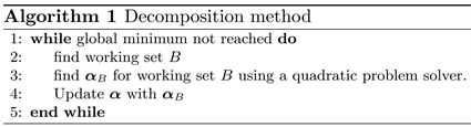
Training dual soft margin SVM requires solving a large scale convex quadratic problem with a linear constraint and simple bounds for variables. To solve large scale SVM problems, decomposition methods such as sequential minimal optimization (SMO) [5] gained popularity due to their efficiency and low memory usage requirement. Each iteration the SMO keeps all the variables except two of them fixed and solves a small two-dimensional subproblem. In an effort to investigate a performance of decomposition based algorithms with larger working sets, one of the previous manuscripts [6] presented an augmented Lagrangian fast projected gradient method (ALFPGM) with working set selection for finding the solution to the SVM problem. The ALFPGM used larger working sets and trained SVM with a size up to 19020 training examples. The current study extends the previous results by presenting an updated working selection method pWSS and testing the improved algorithm on larger data sets with up to tens of thousands of training examples.
The paper is organized as follows. The next section describes the SVM training problem, the ALFPGM and SMO algorithms. Section 3 describes a new working set selection principle responsible for an efficient implementation of ALFPGM. Section 4 provides some details of the calculations. Section 5 provides numerical results. Section 6 contains concluding remarks and Section 7 discusses some future directions of further improving the efficiency of the developed algorithm.
2. SVM Problem
To train the SVM, one needs to find
that minimizes the following objective problem:
(1)
Here
is a set of m labeled data points where
is a vector of features and
represent the label indicating the class to which
belongs. The Matrix Q with the elements
is positive semi-definite but usually dense.
The sequential minimal optimization (SMO) algorithm developed by Platt [7] is one of the most efficient and widely used algorithms to solve (1). It is a low memory usage algorithm that iteratively solves two-dimensional QP subproblems. The QP subproblems are solved analytically. Many popular SVM solvers are based on SMO.
There have been several attempts to further speed up the SMO [8] [9] [10]. In particular, there have been attempts on parallelizing SMO [10]. However, selection of the working set in SMO depends on the violating pairs, which are constantly changed each iteration, making it challenging to develop a parallelized algorithm for the SMO [6]. Other attempts have focused on parallelizing selections of larger working sets of more than one pair. The approach presented here follows the latter path.
2.1. SVM Decomposition
Matrix Q is dense and it is inefficient and often memory prohibitive to populate and store Q in the operating memory for large training data. Therefore decomposition methods that consider only a small subset of variables per iteration [11] [12] are used to train an SVM with a large number of training examples.
Let B be the subset of selected l variables called the working set. Since each iteration involves only l rows and columns of the matrix Q, the decomposition methods use the operating memory economically [11].
The algorithm repeats the select working set then optimize process until the global optimality conditions are satisfied. While B denotes the working set with l variables, N denotes the non-working set with
variables. Then,
, y and Q can be correspondingly written as:
The optimization subproblem can be rewritten as
(2)
with a fixed
. The problem (2) can be rewritten as
(3)
where
and
.
The reduced problem (3) can be solved much faster than the original problem (1). The resulting algorithm is shown as Algorithm 1.
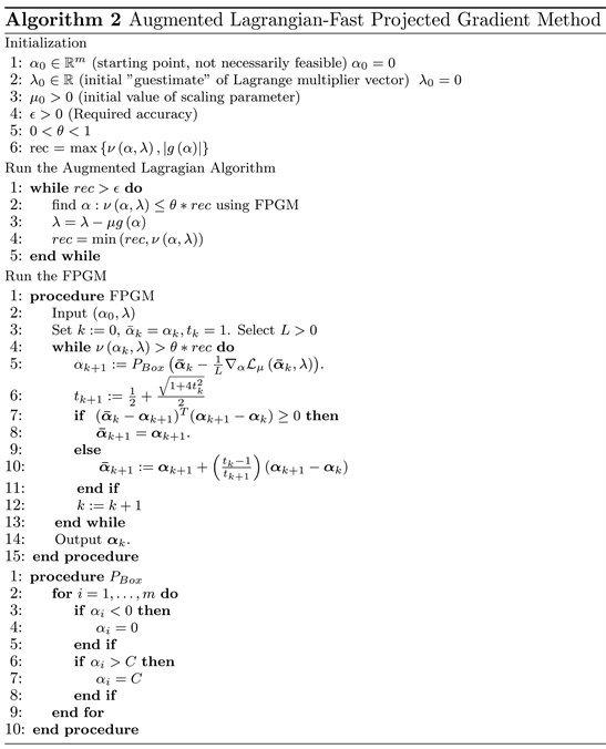
2.2. Augmented Lagrangian—Fast Projected Gradient Method for SVM
A relatively simple and efficient algorithm capable of training medium size SVM with up to a few tens of thousands of data points was proposed in [13]. The algorithm takes advantage of two methods: one is a fast projected gradient method for solving a minimization problem with simple bounds on variables [14] and the second is an augmented Lagrangian method [15] [16] employed to satisfy the only linear equality constraint. The method projects the primal variables onto the “box-like” set:
.
Using the following definitions
(4)
and the bounded set:
(5)
the optimization problem (3) can be rewritten as follows:
(6)
The augmented Lagrangian is defined as
(7)
where
the Lagrange multiplier that corresponds to the only equality constraint and
is the scaling parameter.
The augmented Lagrangian method is a sequence of inexact minimizations of
in
on the
set:
(8)
followed by updating the Lagrange multiplier
:
(9)
The stopping criteria for (8) uses the following function that measures the violation of the first order optimality conditions of (8):
(10)
where
(11)
The minimization (8) (the inner loop) is performed by the fast projected gradient method (FPGM). The inner loop exits when
. The final stopping criteria for the augmented Lagrangian method uses
, which measures the violation of the optimality conditions for (6).
Algorithm 2 describes the ALFPGM (see [6] for more detail). The convergence of Algorithm 2 is established in [17].
3. PWSS Working Set Selection
The flow chart describing pWSS is shown in Figure 1. An important issue of any decomposition method is how to select the working set B. First, a working set selection (WSS) method WSS2nd that uses the second order information [18] is described.
Consider the sets:
Then let us define
In WSS2nd, one selects
(14)
and
(15)
with
where τ is a small positive number.
3.1. Limiting the Search Space for Iup and Ilow
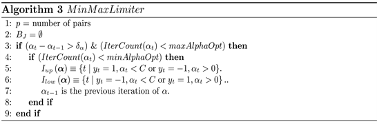
One of the challenges of the previously developed dual decomposition WSS2nd is that a particular data set point can be selected multiple times in different iterations of decomposition in the working set, often increasing the SVM training time. The previously developed algorithm [6] is improved, and the changes to pWSS are made by limiting the search space of Iup and Ilow as described below.
3.2. MinMaxLimiter Algorithm
The MinMaxLimiter algorithm with the following changes to pWSS is proposed:
• Some elements of
that no longer change after many iterations, are eliminated:
, where
,
are two consecutive iterates, and
is a user defined threshold.
• Another introduced parameter is minAlphaOpt, which is the minimum number of times a data index is used in working set. After this threshold, if the value of
is 0 or C, then that data point index is no longer considered
• The last introduced parameter is maxAlphaOpt, which is the maximum number of times a training examples is used in the decomposition rounds.
and
will result in considering every
in every iteration.

3.3. Optimizing j Search Using MinAlphaCheck
Another modification to WSS2nd is the introduction of parameter minAlphaCheck. This is used to reduce the search space of j in (13) to the first minAlphaCheck in the sorted Ilow set. The experimental results show that this converges and is faster than WSS2nd.
4. Implementation
4.1. Kernel Matrix Computation
The cache technique is used to store previously computed rows to access them when the same kernel value needs to be recomputed. The amount of cached kernel is a selectable parameter. The same Least Recently Used (LRU) LRU strategy that SMO implemented in Scikit-learn (Sklearn) was used, and it is a good basis for comparing the results obtained using the SVM training methods. Previous discussions [8] [10] have been held on the ineffectiveness of the LRU strategy. However, that is beyond the scope of this work.
To compute the kernel matrix, Intel MKL is used. The kernel matrix can be computed efficiently using
and the elements of matrix XX', where X is the matrix with the rows made of the data vectors
. Intel MKL’s cblas_dgemv
is used to compute
.
4.2. Computing the Lipschitz Constant L
The Fast Projected Gradient Method (FPGM) requires estimation of the Lipschitz constant L. Since
is of quadratic form with respect to
,
where the matrix spectral norm is the largest singular value of a matrix.
To estimate L first
was estimated. Since
is symmetric and positive semidefinite,
is the largest eigenvalue of
.
The largest eigenvalue
can be efficiently computed using the power method. After estimating
with a few power iterations, the upper bound estimates L as follows:
(16)
5. Experimental Results
For testing, 11 binary classification training data sets (shown in Table 1) were selected with a number of training examples ranging from 18201 to 98528 from University of California, Irvine (UCI) Machine Learning Repository [19] and https://www.openml.org/. One of the tests, Test 2, was the largest test used in the previous work [6]. All simulations were done using a desktop with dual Intel Xeon 2.50 GHz, 12 Cores processors sharing 64 GB of computer memory. In all cases,
was used for all tests. The data was normalized and radial basis kernel was used with
shown in Table 1. The scaling parameter
used for all the experiments is
as suggested in [13]. The parameters in pWSS were taken as
,
,
. The accuracy of solution was selected
. The SVM training times by ALFPGM were compared with results obtained using SMO implemented in Scikit-learn (Sklearn) [20] for the SVM training. The same data inputs were used in SMO and ALFPGM.
ALFPGM—Investigating of Using Different Number of Pairs p
The optimal number of pairs p needed for the training with ALFPGM is determined with numerical experiments using training Tests 2, 6 and 10, which are representatives of small, medium size, and large training sets. In all cases, the pWSS method was employed for the pairs selection. The results are presented in Figures 2-4. The results suggest that for ALFPGM the optimum number of pairs is
.
There are several factors that come into play when varying the number of pairs p.
1) The size of p determines the amount of time it takes to find the size of the working set. The larger the size of p, the longer it takes to find the working set.
2) The smaller the size of p, the more the number of decompositions needed to solve the SVM problem.
3) The larger the size of p, the longer it takes to solve the SVM subproblems.
![]()
Figure 2. ALFPGM—Classification time for different number of pairs p Test 2.
![]()
Figure 3. ALFPGM—Classification time for different numbers of pairs p Test 6.
![]()
Figure 4. ALFPGM—Classification time for different numbers of pairs p Test 10.
4) The larger the size of p, the greater the probability that the Hessian matrix of the SVM subproblem may be degenerate.
Table 2 provides numerical results for training SVM with the ALFPGM and SMO. For each testing dataset, the table shows the number of training examples, the number of features. Then for both ALFPGM and SMO algorithms the table shows the training errors (the fractions of misclassified training examples), the training times, the number of performed decompositions (working set selections), the number of support vectors, and the optimal objective function values. To calculate training times, each simulation scenario was averaged over 5 runs. The results also are visualized in Figures 5-7. The training sets are arranged in the order of increasing the number of training examples. The figures demonstrate that for most of the cases the ALFPGM outperformed the SMO in training time for similar classification error.
Figure 6 shows that the training errors are similar demonstrating that both algorithms produced similar results. The same conclusion can be drawn by observing the similar values of the optimal objective functions for both algorithms in Table 2. Finally, Figure 8 shows the normalized training times i.e. the training times divided by the number of training examples. As one can see, the ALFPGM produces a smaller variance in the normalized times than that of the SMO algorithm.
![]()
Figure 5. Comparison ALFPGM and SMO results timings.
![]()
Figure 6. Comparison ALFPGM and SMO results-training classification error.
![]()
Figure 7. Comparison ALFPGM and SMO results.
![]()
Table 2. ALFPGM and SMO comparison.
![]()
Figure 8. Comparison ALFPGM and SMO normalized time results.
6. Conclusions
The manuscript presents the results on training support vector machines using an augmented Lagrangian fast projected gradient method (ALFPGM) for large data sets. In particular, the ALFPGM is adapted for training using high performance computing techniques. Highly optimized linear algebra routines were used in the implementation to speed up some of the computations.
A working set decomposition scheme for p pairs selection is developed and optimized. Since working set selection takes a large portion of the overall training time, finding an optimal selection of pairs is the key to using multiple pairs in the decomposition. Numerical results indicate that the optimal choice of the number of pairs in the working set p for ALFPGM is 50 - 100 pairs. It is shown that in some examples the selection of pairs can be truncated earlier without compromising the overall results but with significantly reducing training times.
Finally, the comparison of training performance of the ALFPGM with that of the SMO from the Scikit-learn library demonstrates that the training times with ALFPGM is consistently smaller than those for the SMO for the tested large training sets.
7. Future Work
The results demonstrate that the choice of the number of pairs p is important as it determines the number of decompositions. Even though the numerical experiments determined a critical range of values for the optimal value of pairs p, the pWSS can be further improved for multiple pair selection and the total training time will be further reduced.
One possible direction of achieving that improvement is to determine an optimal dependence of the number of pairs p on the size of the training set. Selecting optimal values of WSSminAlphaCheck and minAlphaOpt used in pWSS3 needs to be further explored. Finding the optimal values of ALFPGM parameters based on the input data can further improve the efficiency of the ALFPGM.
A use of graphics processing units (GPU), which are getting less expensive and with more capabilities than before, should be revisited in future. In the future, the most time consuming parts of the algorithm such as computing similarity kernel measures can be done using the GPU.