Generalized Four-Dimensional Scientific CDR Economic Growth Model: Expected Value, Average, and Limits to Growth

Dennis Ridley¹, Felipe Llaugel²

¹School of Business and Industry, Florida A&M University and Department of Scientific Computing, Florida State University, Tallahassee, USA.
²College of Engineering, Universidad Dominicana O&M, Santo Domingo, Dominican Republic.

DOI: 10.4236/tel.[phone]                

Abstract

The parsimonious three-dimensional capitalism, democracy, rule of law (CDR) growth model shows that real per capita gross domestic product (GDP) adjusted for purchasing power parity (GDPppp) is explained almost entirely by only three intangible variables. It is global time invariant. That is, after adjusting for factors of production, capital to GDPppp conversion is the same everywhere in the world, determined by the physical and chemical laws of nature. This paper extends the three-dimensional depiction of the CDR economic growth model to a four-dimensional depiction on a bubble graph, where the bubble size represents GDPppp. The scientific long run expected value of GDPppp growth rate and the limits to growth are derived for the first time. The CDR model is the first and only scientific economic growth model. It places growth economics on a sound scientific footing.

Keywords

Capitalism, Democracy, Rule of Law, Economic Growth

1. Introduction

We know from Ridley (2020a, 2020b) that economic growth is determined by the policy variables capitalism, democracy, rule of law (CDR) model. When natural resources and geography are added to the model, it explains approximately 90% of real per capita gross domestic product (GDP) adjusted for purchasing power parity (GDPppp). The CDR model comprises policy variables C, D and R, and the natural variable N. The model is referred to as the CDR model because only the policy variables C, D and R can be changed while N is determined by nature. The CDR model is global time invariant.

Entrepreneurship is the process of starting a business, typically a startup company offering an innovative product, process or service. The true source of wealth is entrepreneurial capital. Capital comprises intangible exogenous human entrepreneurial ideas of imagination and creativity, and capital stock of knowledge (skills and memory), and tangible endogenous machinery, recordings, computers, etc. A capitalist is one who attempts to maximize one’s earnings in return for one’s efforts. Therefore, every rational person is a capitalist. Capitalism is a method of organizing capital for the purpose of profitable investment. Rule of law is an intangible exogenous catalyst that creates stability for attracting capital. Democracy is an intangible exogenous catalyst that creates new pathways for the optimal deployment of capital. Total capital is converted into production of capital stock, goods and services, which after consumption, depreciation and obsolescence, contributes to wealth. Since capital stock is subject to continuing depreciation and obsolescence, entrepreneurship must be the true source of new wealth creation. Money is a method of accounting for wealth, not the source of wealth. But money and finance are accelerants for promoting a good entrepreneurial idea. The CDR index is a combined weighted average of capitalism (C), democracy (D) and rule of law (R) that jointly with natural resources and geography explain almost all economic growth. It is most impressive how straight the GDPppp vs CDR line is (see Appendix). Also impressive is the small number of variables posited for explaining GDPppp. This is in keeping with the parsimonious principle of Achem’s Razor. We acknowledge this as the CDR scientific law. High CDR countries are where ideas go to fly. Low CDR countries are where ideas go to die.

The novelty of this paper is we extend the Ridley (2020a, 2020b) three-dimensional depiction of the CDR economic growth model (see Appendix) to four dimensions by use of bubble graphing, where the bubble size represents GDPppp. One can observe the evolution of GDPppp as C, D, and R develop. This depiction will show once again that after adjusting for factors of production, capital to GDPppp conversion is the same everywhere in the world, determined by the physical and chemical laws of nature. This is the first ever scientific derivation and computation of the expected value, divergence, curl, and limit to single year economic growth.

The remainder of the paper is organized as follows. The next section is a review of related literature. This is followed by data tabulation and analysis. Regression is then used to parameterize the CDR model, from which we derive the theoretical expected endogenous growth and limits to growth. Finally, we draw conclusions and make suggestions for future research. Because of the novelty of the CDR model, and its unique definitions, a clarifying nomenclature is provided at the end of the paper.

2. Related Literature

Several economic growth models have been proposed. The prominent models include the basic growth models, neo-classical growth models, endogenous growth and an exogenous-endogenous growth model.

Basic growth: The Aggregate Production Function Equation model is an aggregate formulation that is better suited for a microeconomic application. The Saving Equation model assumes that savings is a fixed percentage of income. This assumption fails to be correct over any length of time or across countries. The Relation between Saving and Investment model precludes foreign trade and borrowing. The Change in Capital Stock over Time model incorporates increase in capital over time due to investments and decrease due to depreciation. The Labor Supply Equation model of Harrod (1939) and Domar (1946) is an aggregate formulation of the microeconomic Leontief (1906-1999) production function. It is a Keynesian model of economic growth. It is used in development economics to explain an economy’s growth rate in terms of the level of saving and of capital. It suggests that there is no natural reason for an economy to have balanced growth. The central focus of the Capital-Output Ratio model is on the role of capital accumulation in the growth process.

Neo-classical: The Solow (1956, 1957) model is an aggregate formulation of the microeconomic Cobb & Douglas (1928) production function. The Meade Model (Meade, 1962) is a production function in which the inputs of capital and labor are extended to include land and time trend in technological change. Unlike the neo-classical assumption of ready substitution between capital and labor, in the Kaldor (1957) model all technological change is accompanied by new investment.

Endogenous: The AK Model (Romer, 1986) is one where there are no diminishing returns. This is unlike steady state classical economics (Ricardo, 1817, 1821; Malthus, 1798) and neo-classical economics.

Exogenous-endogenous: The aforementioned models suffer several deficiencies, not the least of which is their low level of accuracy for predicting GDPppp. Ridley and Ngnepieba (2018) gave a mathematical proof that the aggregate production function is ill-conceived and incorrect in that it is a fallacy of composition to think that we can simply jump from microeconomic production function conceptions to an understanding of aggregate production by society as a whole (Cohen and Harcourt, 2003). The exogenous-endogenous CDR model was developed by Ridley (2020a, 2020b). The CDR model explains nearly all (90%) of GDPppp and is therefore the most accurate. This model yields the CDR index that can serve as a guide to economic planners and governments for understanding GDP creation. Only the CDR model incorporates exogenous entrepreneurial human capital ideas of imagination and creativity. Low CDR index countries are doomed to impecuniosity. High CDR index countries are destined for pecuniosity. This model is the focus of this paper.

3. Data

The cross-country data for GDPppp, Capitalization, Democracy and Rule of law are given in Table 1. The data for Natural resources rents and Latitude are given in Table 2. These data are for 79 countries for which a complete set of data is available. Other countries have populations less than one million or simply do not report data. Year 2014 are those given in Ridley (2020a, 2020b) and allows us to make comparisons.

Figure 1 is a four-dimension bubble graph that displays the policy variables C, D, R and the corresponding GDPppp. The sizes of the bubbles are set to GDPppp. As the size increases the bubble color goes from dark blue, to light blue, to green, to yellow, to red, to dark red. As C, D and R increase GDPppp (bubble size)

Click on the bubble graph and wait to see 3 animations (https://sites.google.com/view/cdr4d/home). Scroll down to see how GDPppp evolves contemporaneously with CDR.

Figure 1. Four-dimensional bubble graph: C, D, R and GDPppp (bubble size). These data are for year 2014. Panel data were analyzed for years 1995-2016 and the results were the same, that is global time invariant. For additional comments on the countries listed see Ridley (2017a, 2017b).

Table 1. GDPppp and policy variables: Capitalization per capita (C), Democracy (D), Rule of law (R) by country.

Data sources: GDPppp (constant international$ for 2014, reported by the IMF): http://www.imf.org/external/data.htm. Population: http://data.worldbank.org/indicator/SP.POP.TOTL. Capitalization (US$ mundi): http://www.indexmundi.com/facts/indicators/CM.MKT.LCAP.CD/rankings. Democracy rank: http://democracyranking.org/wordpress/rank/democracy-ranking-2014/. Corruption rank: https://www.transparency.org/research/cpi/. Democracy rank & corruption rank for Bermuda and Honk Kong were set to that for United Kingdom as the governing country. Barbados (high CDR) and Equatorial Guinea (high GDPppp) are too small for attention by the reporting agencies.

Table 2. Nature variables: per capita Natural resource rents (N) and Latitude (L) by country.

Data sources: Total natural resources: http://data.worldbank.org/indicator/NY.GDP.TOTL.RT.ZS. Latitude: La Porta et al. (1999).

tends to increase. The two largest go to Singapore (SG) and Norway (NO) respectively. The capitalizations for Singapore (SG) and Switzerland CH) are atypically very large. Switzerland is unique in its policy with respect to the attraction of capital. The highest goes to Singapore. Singapore is described as a benevolent dictatorship with a low D rating. Its high C and R ratings more than make up for that in determining GDPppp. Its low D rating sets it off the trend in Figure 1. The lowest GDPppp’s go to Malawi (MW) ($1112) and Uganda (UG) (1939).

4. Analysis

The variables in the CDR model are defined as follows:

g = (GDPppp − lowest GDPppp)/(highest GDPppp − lowest GDPppp)

GDPppp = Per capita real gross domestic product adjusted for purchasing power parity

C (Capitalism) = (per capita total market capitalization − lowest per capita total market capitalization)/(highest per capita total market capitalization − lowest per capita total market capitalization)

D (Democracy) = (lowest democracy rank − democracy rank)/(lowest democracy rank − highest democracy rank)

R (Rule of law) = (lowest corruption rank − corruption rank)/(lowest corruption rank − highest corruption rank)

N (Natural resources) = (per capita total natural resource rents − lowest per capita total natural resource rents)/(highest per capita total natural resource rents − lowest per capita total natural resource rents).

L (Latitude) = (Latitude − lowest latitude)/(highest latitude − lowest latitude)

These transformations standardize the variables and ensures upper and lower bounds on 0 ≤ g, C, D, R, CDR, N, L ≤ 1. Data for these standardized variables are listed in Table 1 and Table 2. See Ridley and de Silva (2019) for more on the relationship between corruption and rule of law. Democracy and corruption are rank ordered, where the highest = 1 and the lowest = the number of countries. The inverse transformation of g is GDPppp = g(highest GDPppp − lowest GDPppp) + lowest GDPppp where lowest GDPppp = $1,112 and highest GDPppp = $83,066.

4.1. Parametric Derivation of the Theoretical Expected Endogenous Growth in g

The CDR model comprises policy variables C, D and R, and the natural variable N. Government can change C, D and R, so the model is referred to as the CDR model. N is fixed by nature and cannot be changed. Initially, it was thought that N contributes highly to GDPppp. It turned out that N contributed only 6% to GDP making it much less important than ordinarily considered to be. See the fitted model below. Furthermore, a purpose of CDR is to determine national policy regarding what can be done to raise GDP, and N cannot occur by policy. Therefore, N can be dropped from the model without loss of generality. Still, the following parametric derivation of the theoretical optimal endogenous growth in g includes N for purpose of accuracy in accounting.

The CDR statistical model for GDP is

$g={\beta }_0+{\beta }_{C}C+{\beta }_{D}D+{\beta }_{R}R+{\beta }_{CDR}C\cdot D\cdot R+{\beta }_{N}N+\epsilon$

where all variables are standardized by linear transformation to ensure upper and lower bounds on 0 ≤ g, C, D, R, CDR, N ≤ 1. Democracy and corruption are rank ordered, where the highest = 1 and the lowest = the number of countries. Note that N can be dropped for policy making, leaving just CDR.

The estimated ordinary least squares (OLS) model is

$\begin{array}{l}{\hat{g}}_i=1.53C_i+0.14D_i+0.23R_i-1.21C_i\cdot D_i\cdot R_i+0.38N_i,R_{adj}^2=83\%\\ \left|t\right|=\left(6.6\right)\left(1.7\right)\left(2.6\right)\left(4.5\right)\left(5.6\right)\\ p=59\%5\%10\%3\%6\%\end{array}$

The t statistics indicate that all variables are statistically significant. The partial correlations (p) are the contributions of each variable to $R_{adj}^2$. The largest contribution to explaining g comes from C (59%). The next largest (10%) comes from R. The next largest (5%) comes from D. The next largest (3%) comes from C∙D∙R. The negative coefficient associated with the C∙D∙R term represents the interaction between C, D and R. It is a friction coefficient that subtracts from growth. The friction is debilitating when there is excessive unnecessary democracy due to too much discussion and or excessive unnecessary rule of law due to overregulation. Natural resources N contribute 6% and the intangible CDR policy contributes 59 + 5 + 10 + 3 = 77%. That is, CDR policy contributes 77/6 ≈ 13 times more than natural resources. This reinforces the importance of not relying on natural resources, and focusing on CDR. That is, on how a country is managed.

D_i, R_i, and N_i are exogenous variables. It is obvious that GDPppp cannot influence natural resources so N_i is exogenous. D_i and R_i are catalysts and therefore must be exogenous. To understand this, recognize that as catalysts they increase the production of GDPppp without taking part in the process. Assume for example that at the beginning of the year there is a starting amount of raw materials. Raw materials are used up throughout the year. Therefore, there will be less raw material at the end of the year. But D_i and R_i are not used up by the process. They are the same before and after the process. They are not affected by the process. Therefore, they are exogenous.

C_i comprises exogeneous human ideas of imagination and creation, and endogenous capital stock of knowledge, machines, recordings, etc. For that reason, the above CDR model is biased. Therefore, it is necessary to separate the exogenous and endogenous components of capital. Using latitude measured in L_i units as the instrumental variable for purging endogenous capital from C_i (L_i is correlated with C_i and uncorrelated with ${\epsilon }_i$ and obviously exogenous since GDPppp cannot influence latitude), the estimated model for C_i is

$\begin{array}{l}{\hat{C}}_i=0.04-0.07L_i-0.16D_i+0.22R_i+1.11C_i\cdot D_i\cdot R_i-0.02N_i,R_{adj}^2=95\%\\ \left|t\right|=\left(3.7\right)\left(4.6\right)\left(6.4\right)\left(27.1\right)(\; 0.61\; )\end{array}$

The t statistics indicate that apart from N all variables are statistically significant.

The estimated 2^nd stage least squares model for estimating g from exogenous new idea human capital entrepreneurship ( ${\hat{C}}_i$ ) is

${\hat{g}}_i=1.30{\hat{C}}_i+0.12D_i+0.28R_i-0.98{\hat{C}}_i\cdot D_i\cdot R_i+0.39N_i,R_{adj}^2=74\%$

Therefore, the fraction of total capital that is exogenous entrepreneurship capital = 1.30/1.53 = 0.85 = 85%. Alternatively, the contribution from capital stock is the reduction in $R_{adj}^2$ of 0.83 − 0.74 = 0.09 per unit or 9%, and the contribution of total capital to $R_{adj}^2$ is 0.59. So, the contribution from exogenous entrepreneurship capital is (0.59 − 0.09)/0.59 = 0.85 = 85%. And, capital stock from old ideas that occurred earlier amounts to 15%. See Ridley and Khan (2019) for more on decoupling entrepreneurship capital from capital stock.

The CDR model is designed to get at what a country can do to raise its g. It is limited by data availability for exact computation of average world g. C does not include non-publicly traded private market capital. Those data are not available and will never be available. Still, let us see what CDR predicts for annual g. All the variables in the CDR model are based on per unit values. Therefore, the regression coefficients are the growth in ${\hat{g}}_i$ per unit. So, the purely endogenous growth in g is the expected value of the contribution from the endogenous capital ( $C_i-{\hat{C}}_i$ ) plus the unbiased 2 stage least squares (2SLS) contributions from $D_i,R_i,{\hat{C}}_i\cdot D_i\cdot R_i$ converted to endogenous g via the dot product with the unbiased regression coefficients.

That is, expected endogenous growth in

$g=\left(1/2\right)\left({\hat{\beta }}_0+\left({\hat{\beta }}_C-{\hat{\beta }}_{\hat{C}}\right)+{\hat{\beta }}_D+{\hat{\beta }}_R+{\hat{\beta }}_{\hat{C}DR}+{\hat{\beta }}_N\right)$, where $\hat{\beta }$ denotes estimate of

$\beta$ and (1/2) is the mean of the range [0, 1]. When calculated from the original regression coefficients prior to rounding, ${\hat{\beta }}_C=1.534346$ and ${\hat{g}}_i=-0.00051+$ $1.295617{\hat{C}}_i+0.116963D_i+0.275395R_i-0.98133{\hat{C}}_i\cdot D_i\cdot R_i+0.388146N_i$.

Expected endogenous growth in g = (1/2) (−0.00051 + (1.534346 − 1.295617) + 0.116963 + 0.275395 − 0.98133 + 0.388146) per unit = 0.018698 per unit ≃ 1.8%.

A parametric integral derivation of the theoretical maximum endogenous growth in g is given below.

We mention in passing an interesting observation that this equates to $\frac{1}{4}{e}^2$, where e is the Napier’s constant (Euler’s number) and base for the natural logarithm. While some countries might grow faster than 1.8% others will grow slower than 1.8%. As it turns out this theoretical 1.8% is numerically equal to what economists have observed empirically as the steady state rate to which countries converge as they develop. The developed country per capita g dominance of the world might explain the world proximity to 1.8%. The standard deviation of ${\hat{g}}_i$, ${\sigma }_{{\hat{g}}_i}=0.208513$ per unit. The standard deviation of the mean of g, ${\sigma }_{{\bar{g}}_i}=0.208513/\sqrt{79}=0.02346\simeq 2.3\%$. The plots of the residuals ${\hat{\epsilon }}_i$ versus ${\hat{g}}_i$ from the regression (Figure 2), their histogram (Figure 3) and a chi square goodness of fit test, show that they are approximately random and normally distributed. Therefore, the 95% confidence interval (CI) for the estimate of mean growth in g is

$\text{CI}=1.8\pm \left(z{\sigma }_{{\bar{g}}_i}\right)\%=1.8\pm \left(1.96\times 2.3\right)\%=\left(-2.7\%,6.3\%\right)$.

As best we can tell this derivation of annual endogenous growth rate in g explains the previously observed but unexplained 1.8% and brings that mystery to

Figure 2. Plot of residuals vs. fitted values of g.

Figure 3. Histogram of residuals.

an end. This statistical account is not a scientific explanation per say. But one might speculate that the growth in g is matched to the growth in human population. That is, each child brings its own wealth into the world. A child is an asset not a liability. Furthermore, the child’s discoveries that are exogenous entrepreneurial capital can add to the endogenous growth rate of 1.8%.

See Ridley and de Silva (2019) for a complete set of diagnostic evaluations of the aptness of this CDR model.

4.2. Parametric Integral Derivation of the Theoretical Average g

Consider a spatial analogy and depiction where C_i, D_i and R_i exist in the sphere of influence S in Euclidean space. The purely endogenous element of g is the contribution to flow of gross domestic product through S from the endogenous capital ( $C_i-{\hat{C}}_i$ ) plus the unbiased 2SLS contributions from $D_i,R_i,{\hat{C}}_i\cdot D_i\cdot R_i,N_i$ converted to endogenous g via the dot product with the unbiased regression coefficients. ${\hat{C}}_i$ is exogenous capital and is characteristically different from endogenous capital. Consider g constructed from $C_i,D_i,R_i\in \left[0,1\right]$ for all countries on the sphere (the globe) enclosed by S with a positive orientation with the unit normal vector $\stackrel{\to }{n}$ on the surface S (Figure 4). Consider also a vector field

Figure 4. Subset of volume of g for all countries on a spherical globe. Source: Own schematic.

$\stackrel{\to }{F}$ (C, D, R) whose components are continuously differentiable. We are interested in the flux of $\stackrel{\to }{F}$, flowing globally out of the sphere from the aggregate production systems that create g. Some of g is divergent flow (Gauss, 1777-1855) out of S and some is circular curl (Maxwell, 1831-1879) around the C, D and R axes. The adjacent elements of the neighboring fluxes inside the sphere cancel, leaving a positive total on the boundary. As $C_i,D_i,R_i\le 1$ are set to the values corresponding to a particular country the total for the globe is the one year g for that country. $C_i,D_i,R_i\in \left[0,1\right]$ corresponds to the average annual flow from a hypothetical globe of countries.

The integral of the purely endogenous contribution to the subset of g corresponding to a simple closed CDR space ${ℝ}^n$ (where n = 3), contained in a piecewise smooth boundary of the unit radius sphere and volume g is given by

${\displaystyle {∯}_S\left(\stackrel{\to }{F}\cdot \stackrel{\to }{n}\right)\text{d}S}={\displaystyle {∯}_S\stackrel{\to }{F}\cdot \text{d}\stackrel{\to }{S}}={\displaystyle {\iiint }_V\left(\nabla \cdot \stackrel{\to }{F}\right)\text{d}V}={\displaystyle {\iiint }_{CDR}\left(\nabla \cdot \stackrel{\to }{F}\right)\partial C\partial D\partial R}$

By extension, and for computational accuracy, we include $N_i\in \left[0,1\right]$ in the integral of the purely endogenous contribution to subsetg of a closed CDRN hyperspace ${ℝ}^4$, also contained in a piecewise smooth boundary. The coefficients from the least squares equation for ${\hat{g}}_i$ form the parametrization of $\stackrel{\to }{F}$, and $\stackrel{\to }{F}$ flows outward in all four vector component directions ( $\stackrel{\to }{i}$, $\stackrel{\to }{j}$, $\stackrel{\to }{k}$, $\stackrel{\to }{l}$, positively aligned with C, D, R, and N).

Divergence:

Setting $\stackrel{\to }{F}={\hat{g}}_i={\hat{\beta }}_0+\left({\hat{\beta }}_C-{\hat{\beta }}_{\hat{C}}\right)C_i+{\hat{\beta }}_D{D}_i+{\hat{\beta }}_R{R}_i+{\hat{\beta }}_{\hat{C}DR}{\hat{C}}_i\cdot D_i\cdot R_i+{\hat{\beta }}_N{N}_i$

The flow rate of g though an infinitesimal point of the surface S is given by the divergence

$\nabla \cdot \stackrel{\to }{F}=\partial \stackrel{\to }{F}/\partial C_i+\partial \stackrel{\to }{F}/\partial D_i+\partial \stackrel{\to }{F}/\partial R_i+\partial \stackrel{\to }{F}/\partial N_i$

where $\partial \stackrel{\to }{F}/\partial C_i={\hat{\beta }}_C-{\hat{\beta }}_{\hat{C}}$, $\partial \stackrel{\to }{F}/\partial D_i={\hat{\beta }}_D+{\hat{\beta }}_{\hat{C}DR}{\hat{C}}_i\cdot R_i$, $\partial \stackrel{\to }{F}/\partial R_i={\hat{\beta }}_R+{\hat{\beta }}_{\hat{C}DR}{\hat{C}}_i\cdot D_i$, $\partial \stackrel{\to }{F}/\partial N_i={\hat{\beta }}_N$.

The average of all flows of g from all points of the surface of the global surface representing the production of the world economy is the flux integral

$\begin{array}{l}{\displaystyle {\int }_{N=0}^1{\displaystyle {\int }_{R=0}^1{\displaystyle {\int }_{D=0}^1{\displaystyle {\int }_{C=0}^1\nabla \cdot \stackrel{\to }{F}\partial C\partial D\partial R\partial N}}}}\\ ={\displaystyle {\int }_{N=0}^1{\displaystyle {\int }_{R=0}^1{\displaystyle {\int }_{D=0}^1{\displaystyle {\int }_{C=0}^1\left({\hat{\beta }}_C-{\hat{\beta }}_{\hat{C}}+{\hat{\beta }}_D+{\hat{\beta }}_{\hat{C}DR}{\hat{C}}_i\cdot R_i+{\hat{\beta }}_R+{\hat{\beta }}_{\hat{C}DR}{\hat{C}}_i\cdot D_i+{\hat{\beta }}_N\right)\partial C\partial D\partial R\partial N}}}}\\ ={\displaystyle {\int }_{N=0}^1{\displaystyle {\int }_{R=0}^1{\displaystyle {\int }_{D=0}^1{\left[{\hat{\beta }}_C{C}_i-{\hat{\beta }}_{\hat{C}}{C}_i+{\hat{\beta }}_D{C}_i+{\hat{\beta }}_{\hat{C}DR}{\hat{C}}_i\cdot R_i{C}_i+{\hat{\beta }}_R{C}_i+{\hat{\beta }}_{\hat{C}DR}{\hat{C}}_i\cdot D_i{C}_i+{\hat{\beta }}_N{C}_i\right]}_{C=0}^{C=1}\partial D\partial R\partial N}}}\\ ={\displaystyle {\int }_{N=0}^1{\displaystyle {\int }_{R=0}^1{\displaystyle {\int }_{D=0}^1\left({\hat{\beta }}_C-{\hat{\beta }}_{\hat{C}}+{\hat{\beta }}_D+{\hat{\beta }}_{\hat{C}DR}{\hat{C}}_i\cdot R_i+{\hat{\beta }}_R+{\hat{\beta }}_{\hat{C}DR}{\hat{C}}_i\cdot D_i+{\hat{\beta }}_N\right)\partial D\partial R\partial N}}}\end{array}$

$\begin{array}{l}={\displaystyle {\int }_{N=0}^1{\displaystyle {\int }_{R=0}^1{\left[{\hat{\beta }}_C{D}_i-{\hat{\beta }}_{\hat{C}}{D}_i+{\hat{\beta }}_D{D}_i+{\hat{\beta }}_{\hat{C}DR}{\hat{C}}_i\cdot R_i{D}_i+{\hat{\beta }}_R{D}_i+{\hat{\beta }}_{\hat{C}DR}{\hat{C}}_i\cdot D_i^2/2+{\hat{\beta }}_N{D}_i\right]}_{D=0}^{D=1}\partial R\partial N}}\\ ={\displaystyle {\int }_{N=0}^1{\displaystyle {\int }_{R=0}^1\left({\hat{\beta }}_C-{\hat{\beta }}_{\hat{C}}+{\hat{\beta }}_D+{\hat{\beta }}_{\hat{C}DR}{\hat{C}}_i\cdot R_i+{\hat{\beta }}_R+{\hat{\beta }}_{\hat{C}DR}{\hat{C}}_i/2+{\hat{\beta }}_N\right)\partial R\partial N}}\\ ={\displaystyle {\int }_{N=0}^1{\left[{\hat{\beta }}_C{R}_i-{\hat{\beta }}_{\hat{C}}{R}_i+{\hat{\beta }}_D{R}_i+{\hat{\beta }}_{\hat{C}DR}{\hat{C}}_i\cdot R_i^2/2+{\hat{\beta }}_R{R}_i+{\hat{\beta }}_{\hat{C}DR}{\hat{C}}_i{R}_i/2+{\hat{\beta }}_N{R}_i\right]}_{R=0}^{R=1}\partial N}\\ ={\displaystyle {\int }_{N=0}^1\left({\hat{\beta }}_C-{\hat{\beta }}_{\hat{C}}+{\hat{\beta }}_D+{\hat{\beta }}_{\hat{C}DR}{\hat{C}}_i/2+{\hat{\beta }}_R+{\hat{\beta }}_{\hat{C}DR}{\hat{C}}_i/2+{\hat{\beta }}_N\right)\partial N}\end{array}$

$\begin{array}{l}={\left[{\hat{\beta }}_C{N}_i-{\hat{\beta }}_{\hat{C}}{N}_i+{\hat{\beta }}_D{N}_i+{\hat{\beta }}_{\hat{C}DR}{\hat{C}}_i{N}_i/2+{\hat{\beta }}_R{N}_i+{\hat{\beta }}_{\hat{C}DR}{\hat{C}}_i{N}_i/2+{\hat{\beta }}_N{N}_i\right]}_{N=0}^{N=1}\\ ={\hat{\beta }}_C-{\hat{\beta }}_{\hat{C}}+{\hat{\beta }}_D+{\hat{\beta }}_{\hat{C}DR}{\hat{C}}_i/2+{\hat{\beta }}_R+{\hat{\beta }}_{\hat{C}DR}{\hat{C}}_i/2+{\hat{\beta }}_N\\ ={\hat{\beta }}_C-{\hat{\beta }}_{\hat{C}}+{\hat{\beta }}_D+{\hat{\beta }}_R+{\hat{\beta }}_{\hat{C}DR}{\hat{C}}_i+{\hat{\beta }}_N\end{array}$

Consider the case when ${\hat{C}}_i$ is set to the value estimated from the above 2SLS. That is, when ${\hat{C}}_i=85\%=0.85$. The endogenous capital = 15% and the endogenous g is

$\begin{array}{l}=1.534346-1.295617+0.116963+0.275395-0.98133\left(0.85\right)+0.388146\\ =0.18511\end{array}$

The inverse transformation of g is

GDPppp = g(highest GDPppp − lowest GDPppp) + lowest GDPppp

Where highest lowest GDPppp = $1,112 and highest GDPppp = $83,066

Average GDPppp = 0.18511 ($83,066 − $1,112) + $1,112 = $16,282.50

This flow is close to the average flow obtained from the observed data in Table 1 and Table 2.

Total gross domestic product divided by total population = (22,302 × 1,971,300 + 8164 × 5,939,993 +…+ 5656 × 91,700,000)/(1,971,300 + 5,939,993 +…+ 91,700,000) = $16,940.34.

Different flows would result from different combinations of C, D, R and N.

Curl:

The curl of the circulations in the positive D-R, C-R and C-D planes represent what is analogous to turbulence. They are inefficiencies relative to the desired outward flow. These are the results of such activity as circulating ideas that gain no traction for whatever reason. Ideas and activities going in circles if you will. They involve an over democratized process of excessive discussion and overthinking. Over democratization results in unnecessary delays and loss of opportunity. There is also the possibility of excessive regulation. Overregulation results in the prevention of opportunity.

Consider the three-dimensional curl of $\stackrel{\to }{F}$. The variable $N_i$ does not appear in the interactive ${\hat{C}}_i\cdot D_i\cdot R_i$ term so, there is no curl involving N.

$\begin{array}{l}Curl\stackrel{\to }{F}=\nabla \times \stackrel{\to }{F}=\left|\begin{array}{ccc}\stackrel{\to }{i}& \stackrel{\to }{j}& \stackrel{\to }{k}\\ \partial /\partial C& \partial /\partial D& \partial /\partial R\\ {\stackrel{\to }{F}}_C& {\stackrel{\to }{F}}_D& {\stackrel{\to }{F}}_R\end{array}\right|\\ =\left(\partial \stackrel{\to }{F}/\partial D_i-\partial \stackrel{\to }{F}/\partial R_i\right)\stackrel{\to }{i}-\left(\partial \stackrel{\to }{F}/\partial C_i-\partial \stackrel{\to }{F}/\partial R_i\right)\stackrel{\to }{j}+\left(\partial \stackrel{\to }{F}/\partial C_i-\partial \stackrel{\to }{F}/\partial D_i\right)\stackrel{\to }{k}\end{array}$

Once again setting $\stackrel{\to }{F}={\hat{g}}_i={\hat{\beta }}_0+\left({\hat{\beta }}_C-{\hat{\beta }}_{\hat{C}}\right)C_i+{\hat{\beta }}_D{D}_i+{\hat{\beta }}_R{R}_i+{\hat{\beta }}_{\hat{C}DR}{\hat{C}}_i\cdot D_i\cdot R_i$ $+{\hat{\beta }}_N{N}_i$

$\begin{array}{l}=\left({\hat{\beta }}_D+{\hat{\beta }}_{\hat{C}DR}{\hat{C}}_i\cdot R_i-{\hat{\beta }}_R-{\hat{\beta }}_{\hat{C}DR}{\hat{C}}_i\cdot D_i\right)\stackrel{\to }{i}-\left({\hat{\beta }}_C-{\hat{\beta }}_{\hat{C}}-{\hat{\beta }}_R-{\hat{\beta }}_{\hat{C}DR}{\hat{C}}_i\cdot D_i\right)\stackrel{\to }{j}\\ +\left({\hat{\beta }}_C-{\hat{\beta }}_{\hat{C}}-{\hat{\beta }}_D-{\hat{\beta }}_{\hat{C}DR}{\hat{C}}_i\cdot R_i\right)\stackrel{\to }{k}\end{array}$

$\begin{array}{c}Curl\stackrel{\to }{F}=\left(0.11696-0.98133{\hat{C}}_i{R}_i-0.275395354+0.98133{\hat{C}}_i{D}_i\right)\stackrel{\to }{i}\\ -\left(1.534346-1.295617-0.275395354+0.98133{\hat{C}}_i{D}_i\right)\stackrel{\to }{j}\\ +\left(1.534346-1.295617-0.116963+0.98133{\hat{C}}_i{R}_i\right)\stackrel{\to }{k}\end{array}$

Consider C = D = R = 1 for all countries, ${\hat{C}}_i=0.85$, then

$\begin{array}{c}Curl\stackrel{\to }{F}=\left(0.11696-0.98133\left(0.85\right)-0.275395354+0.98133\left(0.85\right)\right)\stackrel{\to }{i}\\ -\left(1.534346-1.295617-0.275395354+0.98133\left(0.85\right)\right)\stackrel{\to }{j}\\ +\left(1.534346-1.295617-0.116963+0.98133\left(0.85\right)\right)\stackrel{\to }{k}\end{array}$

$Curl\stackrel{\to }{F}=-0.16\stackrel{\to }{i}-0.80\stackrel{\to }{j}+0.96\stackrel{\to }{k}$

$\text{Thedivergenceof}Curl\stackrel{\to }{F}=\nabla \cdot Curl\stackrel{\to }{F}=-0.16-0.80+0.96=0$.

Ideally, we would like there to be no curl ( $0\stackrel{\to }{i}+0\stackrel{\to }{j}+0\stackrel{\to }{k}$ ). In practice however and in this example, there are inefficiencies due to the curl of positive and negative circulations. The sum of these curls is zero, resulting in no contribution to production as measured by flow out of S.

The smallest curl (−0.16) is around lines parallel to the positive C axis. This suggests negative D-R interactions. This suggests overthinking and overregulation that cause delayed decision making and lost or blocked opportunity. The next curl (−0.8) is around lines parallel to the positive D axis. This suggests negative C-R interactions. This suggests overregulation or inappropriate regulations that prevent capital attraction, and block opportunity. The next curl (0.96) is around lines parallel to the positive R axis. This suggests positive C-D interactions. This suggests overthinking with regard to the deployment of the stock of fixed endogenous capital. Efficiency is also limited by the laws of science as is common for physical and chemical processes. These curls represent investment, and inefficiencies that combine to cancel what might otherwise have been contribution to production as measured by flow out of S.

4.3. Parametric Integral Derivation of the Theoretical Maximum Endogenous Growth in g

The integral of the purely endogenous contribution to subset g of a simple closed CDR space ${ℝ}^n$ (where n = 3), contained in a piecewise smooth boundary of the volume g:

$={\displaystyle {\oint }_{CDR}\text{endogenous contribution to}g\partial C\partial D\partial R}$.

By extension, and for computational accuracy, we include $N_i\in \left[0,1\right]$ in the integral of the purely endogenous contribution to subset g of a closed CDRN hyperspace ${ℝ}^4$, also contained in a piecewise smooth boundary:

$\begin{array}{l}{\displaystyle {\oint }_{CDRN}\text{endogenous contribution to}g\partial C\partial D\partial R\partial N}\\ ={\displaystyle {\int }_{N=0}^1{\displaystyle {\int }_{R=0}^1{\displaystyle {\int }_{D=0}^1{\displaystyle {\int }_{C=0}^1\left({\hat{\beta }}_0+\left({\hat{\beta }}_C-{\hat{\beta }}_{\hat{C}}\right)C_i+{\hat{\beta }}_D{D}_i+{\hat{\beta }}_R{R}_i+{\hat{\beta }}_{\hat{C}DR}{\hat{C}}_i\cdot D_i\cdot R_i+{\hat{\beta }}_N{N}_i\right)\partial C\partial D\partial R\partial N}}}}\\ ={\displaystyle {\int }_{N=0}^1{\displaystyle {\int }_{R=0}^1{\displaystyle {\int }_{D=0}^1{\left[{\hat{\beta }}_0{C}_i+\left({\hat{\beta }}_C-{\hat{\beta }}_{\hat{C}}\right)C_i^2/2+{\hat{\beta }}_D{D}_i{C}_i+{\hat{\beta }}_R{R}_i{C}_i+{\hat{\beta }}_{\hat{C}DR}{\hat{C}}_i\cdot D_i\cdot R_i{C}_i+{\hat{\beta }}_N{N}_i{C}_i\right]}_{C=0}^{C=1}\partial D\partial R\partial N}}}\\ ={\displaystyle {\int }_{N=0}^1{\displaystyle {\int }_{R=0}^1{\displaystyle {\int }_{D=0}^1\left({\hat{\beta }}_0+\left({\hat{\beta }}_C-{\hat{\beta }}_{\hat{C}}\right)/2+{\hat{\beta }}_D{D}_i+{\hat{\beta }}_R{R}_i+{\hat{\beta }}_{\hat{C}DR}{\hat{C}}_i\cdot D_i\cdot R_i+{\hat{\beta }}_N{N}_i\right)\partial D\partial R\partial N}}}\\ ={\displaystyle {\int }_{N=0}^1{\displaystyle {\int }_{R=0}^1{\left[{\hat{\beta }}_0{D}_i+\left({\hat{\beta }}_C-{\hat{\beta }}_{\hat{C}}\right)D_i/2+{\hat{\beta }}_D{D}_i^2/2+{\hat{\beta }}_R{R}_i{D}_i+{\hat{\beta }}_{\hat{C}DR}{\hat{C}}_i\cdot D_i^2\cdot R_i/2+{\hat{\beta }}_N{N}_i{D}_i\right]}_{D=0}^{D=1}\partial R\partial N}}\end{array}$

$\begin{array}{l}={\displaystyle {\int }_{N=0}^1{\displaystyle {\int }_{R=0}^1\left({\hat{\beta }}_0+\left({\hat{\beta }}_C-{\hat{\beta }}_{\hat{C}}\right)/2+{\hat{\beta }}_D/2+{\hat{\beta }}_R{R}_i+{\hat{\beta }}_{\hat{C}DR}\cdot {\hat{C}}_i\cdot R_i/2+{\hat{\beta }}_N{N}_i\right)\partial R\partial N}}\\ ={\displaystyle {\int }_{N=0}^1{\left[{\hat{\beta }}_0{R}_i+\left({\hat{\beta }}_C-{\hat{\beta }}_{\hat{C}}\right)R_i/2+{\hat{\beta }}_D{R}_i/2+{\hat{\beta }}_R{R}_i^2/2+{\hat{\beta }}_{\hat{C}DR}\cdot {\hat{C}}_i\cdot R_i^2/4+{\hat{\beta }}_N{N}_i{R}_i\right]}_{R=0}^{R=1}\partial N}\\ ={\displaystyle {\int }_{N=0}^1\left({\hat{\beta }}_0+\left({\hat{\beta }}_C-{\hat{\beta }}_{\hat{C}}\right)/2+{\hat{\beta }}_D/2+{\hat{\beta }}_R/2+{\hat{\beta }}_{\hat{C}DR}\cdot {\hat{C}}_i/4+{\hat{\beta }}_N{N}_i\right)\partial N}\\ ={\left[{\hat{\beta }}_0{N}_i+\left({\hat{\beta }}_C-{\hat{\beta }}_{\hat{C}}\right)N_i/2+{\hat{\beta }}_D{N}_i/2+{\hat{\beta }}_R{N}_i/2+{\hat{\beta }}_{\hat{C}DR}\cdot {\hat{C}}_i\cdot N_i/4+{\hat{\beta }}_N{N}_i^2/2\right]}_{N=0}^{N=1}\\ ={\hat{\beta }}_0+\frac{{\hat{\beta }}_C-{\hat{\beta }}_{\hat{C}}}{2}+\frac{{\hat{\beta }}_D}{2}+\frac{{\hat{\beta }}_R}{2}+\frac{{\hat{\beta }}_{\hat{C}DR}\cdot {\hat{C}}_i}{4}+\frac{{\hat{\beta }}_N}{2}\end{array}$

Consider the case when ${\hat{C}}_i$ is set to the value estimated from the above 2SLS. That is, when ${\hat{C}}_i=85\%=0.85$. The endogenous capital = 15% and the endogenous contribution to g:

$\begin{array}{l}=-0.00051+\frac{1.534346-1.295617}{2}+\frac{0.116963}{2}+\frac{0.275395}{2}\\ +\frac{-0.98133\left(0.85\right)}{4}+\frac{0.388146}{2}\\ =0.3\simeq 30\%\end{array}$

This result is a theoretical maximum conversion of C, D, R, N contributions to g in one year. The high value 0.3 per unit = 30% is due to the negative CDR friction component being reduced by dividing it by 4, while the C, D, R, N components are divided by only 2. It implies that if the democratic decision-making process can be sped up while considering all points of view, the deployment of C can be such that the annual endogenous growth rate in g is 30%.

This is the theoretical largest one-year growth rate. The number is surprisingly large. But very large changes have actually occurred in the past. The biggest actual annual drop in GDP in the history of the United States of America (USA) occurred in 1932. The economy contracted (−12.9%) during the worst year of the great depression. The highest numbers since 1929 for the USA were 17.7% in 1941, 18.9% in 1942, 17.0% in 1943. In 1994, GDP per capita in Armenia was $400. Rapid economic growth occurred in the country in the 2000’s due to a boom in construction. GDP per capita reached $4010 in 2008. That is a 14-year annual growth rate of approximately 18%. The world’s highest change occurring so far was 25% in Libya in 2017. This year 2022, the USA and its North Atlantic Treaty Organization (NATO) and other worldwide partners applied the maximum possible sanctions to Russia and the value of the ruble and GDP fell 30%.

4.4. Discussion

It is recognized that below a certain growth (value unknown) in g, the economy remains stable. When the system is perturbed, the related endogenous economic variables act and interact so as to return the economy to its equilibrium condition. Economics has no precise definition of overheating. But it is also recognized that sustained high growth in g, due to some exogenous government policy intervention say, can lead to the condition where there is more demand for goods and services than can be supplied by the economy. This can lead to price inflation, reaching a point where a reduction in g does not by itself correct the condition and end inflation. This condition of instability is referred to as overheating. The above theoretical maximum single year endogenous percentage growth rate in g may be plausible for infinitesimally small changes in C, D, R, N. However, due to physical limitations, the economy would begin to overheat long before the sustained growth rate in g approaches this value. We do not expect it to be a practical sustainable rate because it is so much higher than the parametrically derived long run theoretical statistical expected endogenous growth rate in g of 1.8% calculated above.

5. Conclusion

The theoretical expected rate in GDPppp is 1.8%. Underdeveloped countries may have lower and even negative growth rates. Developing countries may have a higher growth rate while they catch up, especially since the base for computation is low. As the country develops the growth will approach 1.8%. For example, such are the cases of Canada, Germany and the United States of America. To raise GDPppp a country must raise its CDR profile. It is well known that 10% of the people in the world are rich and getting richer while 90% are impecunious. Efforts to raise the CDR profile of those countries that remain poor are perfunctory at best.

The fraction of capital in the economy that is exogenous human ideas of creativity and imagination is 85%. The endogenous fraction is 15%. The world average expected GDPppp for year 2014 (selected to permit comparisons to other research on the same data) in this study was $16,282.50. This flow was accompanied by inefficiencies due to unproductive circulations of effort on account of overthinking and overregulation. The CDR model is global time invariant, therefore the average can be calculated for any year for which the maximum and minimum GDPppp are known. For the first time, this paper shows that there is a maximum limit to endogenous growth of 30% that can occur in any one year. If this limit were to be approached in more than one successive year, instability would occur before long. We end by noting that the growth rate in GDPppp where economic instability begins has never been formally calculated in the field of economics. A study on the dynamics of instability would be a most worthwhile endeavor.

Acknowledgements

The authors would like to thank Pierre Ngepieba and Paul Beaumont for helpful comments and good discussions.

Significance

The first ever scientific derivation and computation of the expected value and limit to single year economic growth are presented.

Nomenclature

Capital (source): See human capital.

Capitalist: One who deploys one’s personal capital so as to maximize one’s benefit.

Capital stock: Fixed installed capital less depreciation and obsolescence plus skills and knowledge acquired from entrepreneurs and taught to others.

Capitalism: Mechanism for the collection and assembly of capital.

Catalysis:The creation of alternative pathways to enable a process.

CDR index: The vector inner product (dot product) of the global constant [1.53 0.14 0.23 -1.21] and the country [C D R C∙D∙R].

Collaboration: The plan and execution thereof by participants for their intentional mutual benefit of shared goals, objectives, and rewards.

Company: The instrument of capitalism for the profitable investment of capital.

Cooperation: A plan and execution thereof by participants, each with their own personal self-interest and economic gain in mind yet yielding unintended mutual benefits.

Democracy: Private work force idea participation and periodic election of public representatives (catalyst for the process of generating G from capital).

Economic development: The improvement in infrastructure and social wellbeing.

Economic growth: The improvement in per capita real gross domestic product adjusted for purchasing power parity.

Endogenous: Generated from within a system.

Entrepreneurship: The process of starting a business, typically a startup company offering an innovative product, process or service.

Exogenous: Generated from outside a system.

Gross domestic product: The monetary value of all the finished goods and services produced within a country’s borders in a specific time period (economic growth = change in GDP).

Growth in Wealth:Gross domestic product less consumption, depreciation and obsolescence.

Human capital:Capital human ideas of imagination and creativity and skill (not including physical corporeal labor).

Human labor:Physical corporeal labor (not including capital human ideas of imagination and creativity or skill).

Limited liability: Limitation of loss to capital invested.

Natural resources rents: Surplus value of natural resources after all costs and normal returns are accounted for.

Normal distribution: A distribution containing a most frequently occurring typical score at its peak (center) and atypical scores with lower and lower frequency as they occur further and further away from the mean.

Property rights:Property is a legal expression of an economically meaningful consensus by people about assets, how they should be held, used and exchanged.

Rule of Law: Reverse of corruption (protection of shareholder and other property rights) (catalyst for the attraction of capital).

Shareholder: An owner of shares in a company.

Virtue: Self-governing human property that promotes fairness and justice without the need for central government.

Appendix

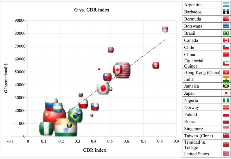
Year 2014 G vs CDR Index for 79 countries (line). Bubble size (21 countries) is the square root of population. This model was re-estimated for panel data and individual years 1995 to 2016 with similar results. For additional comments on the countries listed see Ridley (2017a, 2017b).

Conflicts of Interest

The authors declare no conflicts of interest regarding the publication of this paper.

References

[1]	Cobb, C. W., & Douglas, P. H. (1928). A Theory of Production. American Economic Review, 18, 139-165.
[2]	Cohen, A. J., & Harcourt, G. C. (2003). Retrospectives: Whatever Happened to the Cambridge Capital Theory Controversies? Journal of Economic Perspectives, 17, 199-214. https://doi.org/10.1257/089533003321165010
[3]	Domar, G. (1946). Capital Expansion, Rates of Growth and Employment. Econometrica, 14, 137-147. https://doi.org/10.2307/1905364
[4]	Gauss, C. F. (1777-1855). Carl Friedrich Gauss—Wikipedia.
[5]	Harrod, F. (1939). An essay in Dynamic Theory. Economic Journal, 49, 19-33. https://doi.org/10.2307/2225181
[6]	Kaldor, N. (1957). A Model of Economic Growth. Economic Journal, 69, 591-624. https://doi.org/10.2307/2227704
[7]	La Porta, R., Lopez-de-Silanes, F., Shleifer, A., & Vishny, R. (1999). The Quality of Government. Journal of Law, Economics and Organization, 15, 222-279. https://doi.org/10.1093/jleo/15.1.222
[8]	Leontief, W. (1906-1999). Leontief Production Function. Wikipedia. https://en.wikipedia.org/wiki/Leontief_production_function.
[9]	Malthus, T. R. (1798). An Essay on the Principle of Population. Pelican Books.
[10]	Maxwell, J. C. (1831-1879). James Clerk Maxwell—Wikipedia. https://en.wikipedia.org/wiki/James_Clerk_Maxwell
[11]	Meade, J. E. (1962). A Neoclassical Theory of Economic Growth. Allen & Unwin.
[12]	Ricardo, D. (1817). On the Principles of Political Economy and Taxation. J.M. Dent & Sons, 1911, Dover, 2004.
[13]	Ricardo, D. (1821). The Principles of Political Economy and Taxation. Dent.
[14]	Ridley, A. D. (2017a). Wealth Is All in the Mind. International Journal of Social Science & Economic Research, 2, 3369-3379. http://ijsser.org/uploads/ijsser_02__208.pdf
[15]	Ridley, A. D. (2017b). Division of Human Capital Creates Surplus Wealth. Bulletin of Political Economy, 11, 1-20. https://bulletinofpe.com/
[16]	Ridley, A. D., & Ngnepieba, P. (2018). Conservation of Capital: Homeomorphic Mapping from Intangible Aggregate Macro-Economic CDR Space into Tangible Micro-Economic Production Spaces. Theoretical Economics Letters, 8, 2103-2115. https://doi.org/10.4236/tel.[phone]
[17]	Ridley, A. D., & Khan, A. (2019). Decoupling Entrepreneurship Capital from Capital Stock. Bulletin of Political Economy, 13, 77-86.
[18]	Ridley, A. D., & de Silva, A. (2019). Game Theoretic Choices between Corrupt Dictatorship Exit Emoluments and CDR Benefits: Is There a Nash Equilibrium? The American Economist, 65, 51-77. https://doi.org/10.1177/0569434519878858
[19]	Ridley, A. D. (2020a). Capitalism/Democracy/Rule of law Interactions and Implications for Entrepreneurship and Per Capita Real Gross Domestic Product Adjusted for Purchasing Power Parity. Journal of the Knowledge Economy, 12, 384-411. https://doi.org/10.1007/s13132-020-00632-6
[20]	Ridley, A. D. (2020b). The Mystery of Wealth: Capitalism. Democracy. Rule of Law. Sciendo (De Gruyter). https://content.sciendo.com/search?pageSize=10&q1=The+Mystery+of+Wealth&sort=relevance&subSite=sciendo https://www.amazon.com/s?k=the+mystery+of+wealth+by+ridley&ref=nb_sb_noss
[21]	Romer, P. M. (1986). Increasing Returns and Long-Run Growth. Journal of Political Economy, 94, 1002-1037. https://doi.org/10.1086/261420
[22]	Solow, R. M. (1956). A Contribution to the Theory of Economic Growth. Quarterly Journal of Economics, 70, 65-94. https://doi.org/10.2307/1884513
[23]	Solow, R. M. (1957). Technical Change and the Aggregate Production Function. Review of Economics and Statistics, 39, 312-320. https://doi.org/10.2307/1926047