Geospatial Analysis and Modeling of Indoor Air Quality in Some Residential Areas in the Niger Delta, Nigeria ()
Highlights of Study
· The concentration of CO, SO2, and NO2 was high in indoor and outdoor areas.
· Proximity to the road influenced concentration of noxious gases in Port Harcourt City.
· High-density areas have more concentration of noxious gases than low-density areas.
· Seasons influenced the concentration of noxious gases in indoor and outdoor areas.
· Model showed high correlation between predicted and measured values of pollutants.
1. Introduction
Life has significantly increased in abundance, complexity, and diversity over the earth’s history but has continuously altered the earth’s environment, posing a severe threat to earth’s inhabitants (Kleidon, 2010). According to Shikazono (2012), the atmosphere, hydrosphere, and lithosphere make up the earth’s system. While the atmosphere itself is composed of the following molecules: nitrogen (78%), oxygen (21%), argon (1%), and then trace amounts of carbon dioxide, neon, helium, methane, krypton, hydrogen, nitrous oxide, xenon, ozone, iodine, carbon monoxide, ammonia, and quantities of water vapour at lower altitudes (Hu et al., 2022; Saha, 2008).
According to Chernyaeva and Wang (2019), air pollution is generally referred to as the introduction of chemical, biological and physical substances into the air, thereby altering the air’s natural concentration. Harmful gases cause air pollution, and so impact the atmospheric equilibrium. Some activities that cause this situation are burning coal, oil, and natural gas.
The industrialization process involves converting raw materials into valuable products and waste (Babla et al., 2022), and when the waste is released, it affects the environmental quality (Bhat et al., 2022). Anthropogenic activities such as deforestation, movement of vehicles, building construction, agriculture, construction of roads, and road traffic congestion have also impacted the eco-environment. According to Breysse et al. (2010), air pollution inside homes consists of a complex mixture of agents penetrating from outdoor air and agents generated by indoor sources that have the potential of causing significant health implications.
The primary sources of indoor air pollution worldwide can be attributed to the combustion of fuels, tobacco, coal, ventilation systems, emissions from furnishings and construction materials (Pérez-Padilla et al., 2010; Wu et al., 2022). Indoor fires can produce black carbon particles, nitrogen oxides, sulphur oxides, and mercury compounds, among other emissions (Apte & Salvi, 2016).
WHO (2006) reported that over 1.6 million people died from cooking stove fumes globally (Patha et al., 2017). About 396,000 of the 1.6 million deaths occurred in sub-Sahara Africa, with Nigeria having the highest incidents (Margulis et al., 2006). Health complications emanating from indoor air pollution (IAP) include pneumonia in children, asthma, tuberculosis, upper airway cancer, and cataract (Omole & Ndambuki, 2014). According to Margulis et al. (2006), other familiar sources of IAP include mosquito repellent fumes, electricity generator fumes, and smoke from cigarettes. There has been a rapid increase in generators over the past decade as an alternative source of power for homes and commercial activities in Nigeria (Onwuka et al., 2017). The use of generators has led to high concentrations of carbon monoxide (CO), nitrogen dioxide (NO2), and sulphur dioxide (SO2) in the atmosphere (Sulaiman et al., 2017). Carbon monoxide (CO) is a very hazardous, colorless, and odourless gas emitted from incomplete combustion of fuel in power generator sets, automobiles, and firewood. Global data shows that indoor air pollution (IAP) is far more lethal than outdoor air pollution (OAP) (Omole & Ndambuki, 2014). The objective of the current study is to assess and compare the indoor air quality (IAQ) over different residential categories in Port Harcourt Metropolis, and (2) to forecast dry and wet season indoor and outdoor air quality in both high- and low-density areas.
Research Structure
To achieve the above objectives, the research structure was outlined by studying forty residential areas, which were georeferenced and the density of population delineated into high and low and placed in geospatial maps with GPS. The gaseous samples (SO2, NO2 and CO), the dependent variables, were taken with gas monitors at indoor and outdoor environment, in low and high density aareas during the dry and wet seasons (independent variables) (Figure 2).
2. Materials and Methods
2.1. Description of Study Area
Port Harcourt is the capital city of River Sate (Figure 1) in the Niger Delta region of Nigeria (Ayotamuno & Gobo, 2004, Echendu & Georgeou, 2021). It lies along Bonny River, an eastern tributary of the Niger River, 66 km upstream from the Gulf of Guinea, located in the coastal region. Port Harcourt metropolis partly situated in a wetland ecosystem between Latitudes 4˚45'N, and 4˚55'N and Longitudes 6˚55'E and 7˚05'E with 15.83 meters elevation above sea level (Yakubu, 2018).
The city has a flat topography with an inadequate drainage facility. Its elevation varies between 3 m and 15 m above mean sea level. The stream is a south-flowing stream, turbid during the wet season due to the discharge of clay and silt into the drainage channels. However, the water discharge and turbidity are reduced during the dry season.
Port Harcourt has been under the sub-equatorial climate and experiences a more extended rainy season, characteristic of a tropical wet climate (Numbere, 2022). This climate often experiences lengthy and heavy rainy seasons of about 182 days with a temporary cessation of rain within the rainy season, commonly referred to as “August break” and short dry seasons (Numbere & Camilo, 2018).
2.2. Research Design
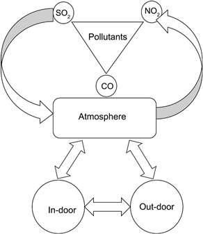
The conceptual model below shows a hypothetical relationship between the main ideas of the study (Figure 2). The independent variables are categorical because they are not continuous numerical data. They are rather the factors that control the dependent variables, which is the gaseous concentrations (SO2, NO2 and CO). For instance, seasons influence gaseous concentration and determine whether it will be high or low. Similarly, the intervening variables (structure of the residences and type of equipments used, distance from road etc) have a role to play in the concentration of the noxious gases (See Figure 2 for details).
2.3. Sample Collection
We used a Garmin GPS (Model 76Cx) to take the coordinates of the sampling points. We also used a gas monitor (Aero qual series 500) to assess the gaseous pollutants in forty (40) residences in the study area (TableA1). The gas monitor is a portable meter with highly sensitive replaceable sensors of different gaseous air pollutants. We then used a portable meter to measure the three gases, namely: Sulphur Dioxide (SO2), Carbon Monoxide (CO), and Nitrogen Dioxide (NO2), by the principle of light absorption and emission. Nitrogen Dioxide (NO2), has 0.001 ppm detection limit, while Sulphur Dioxide (SO2) and Carbon Monoxide (CO) have 0.01 ppm detection limit. The infra-red wavelength of the parameters is not the same.
![]()
Figure 2. Model for the operationalization of the variable in the research.
2.4. Statistical Analysis
Data were analyzed using geospatial and geostatistical techniques with the mean values of the air pollutant concentrations estimated for measurement collected. Statistical test of significance was estimated as the null hypothesis for significance testing. The mean, standard deviations, and coefficient of variations were also calculated. The P-value represents the probability associated with the outcome of a test of a null hypothesis (Bowling, 2014). A normality test was carried out to determine whether the data followed a normal distribution. An analysis of variance (ANOVA) was done to determine the significant difference between multiple locations and sampling units (Logan, 2010). Mann-Whitney test of significance was used to compare the air quality between the high-density area and the low-density area. All analyses were done in R Development Core Team (2013).
2.5. Determination of Indoor Air Quality Index (IAQI)
The indoor air quality index (IAQI) was determined using the existing air quality index (IAQI) (USEPA, 2003) as shown in Equation (1).
(1)
where:
Ip = Index value for pollutant p,
Cp = Rounded concentration of pollutant p,
BPHi = Higher Breakpoint value of Cp,
BPLo = Lower Breakpoint value of Cp,
IHi = Index Breakpoint value of BPHi,
ILo = Index Breakpoint value of BPLo.
2.6. Method of Geospatial Analysis
An ArcGIS 10.2 software was used to map the indoor air quality contours. This software is a Geographic Information System program that integrates spatial data and attributes (indoor air quality values), stores them, and analyses input variables for graphic presentation.
2.7. Modelling Indoor Air Quality
This indoor modelling uses a mass balance approach to estimate indoor air pollutant concentrations in the study area. It is based on indoor modelling techniques used by Davis and Cornwell (2008). In this modelling approach, a house was considered a simple box, as shown in Figure 3. The air quality standards and the reference pollutant limits are in Table A2 and Table A3.
![]()
Figure 3. Mass balance for indoor air quality modeling.
The governing mass balance model for indoor air pollution as contained in Davis and Cornwell (2008) is expressed as given in Equation (2)
(2)
where, C = concentrations (μg/m3);
Ca = ambient concentrations (μg/m3);
Q = rate of infiltration of air into and out of box (m3/s);
V = volume of box (m3);
E = emission rate of pollutant into box from indoor source (g/s);
k = pollutant decay constant or rate of reaction coefficient (/s).
Volume of Box (V)
The average dimensions of rooms measured in the high-density area are 3.5 m × 3.5 m × 6 m = 73.5 m3. Therefore, V for the high-density area was assumed to be 75 m3. The average dimensions of rooms measured in the low-density area are 9 m × 4.6 m × 6 m = 248.4 m3, whereV for the low-density area was assumed to be 250 m3. The reaction rate of coefficient, k, is given as 0.0/s for CO, 4.17 × 10⁻⁵ for NO2, and 6.39 × 10⁻⁵ for SO2. For conservative purposes, the rate of air infiltration into and out of the box, Q, was assumed to be 0.025 m3/s at the same time, the taken modelling time is t = 1 hour (3600 s).
3. Results
3.1. Spatial Interpolation of Air Pollutant Concentrations in the Study Area
The indoor concentrations of air pollutants in both the high-density and low-density areas and during the dry and wet seasons were spatially interpolated to estimate indoor air pollutants. The spatial interpolation was carried out on three criteria pollutants of SO2, NO2, and CO. The global pollutants limits were used as reference points for this study (See Tables A1-A4). The interpolation maps of spatial distribution of the gases are shown in Figures 4(A)-(F). The maps in Figure 4 shows that there is gradual reduction of SO2 and NO2 from high density area to low density areas for both dry and wet seasons (Figures 4(A)-(D))
![]()
Figure 4. Spatial interpolation of indoor SO2 for dry and wet seasons (A and B); NO2 for wet and dry Season (C and D) and CO for dry and wet season (E and F). (Source: by authors).
while in contrast it is the opposite for CO where there was a graual reduction of cocnetrion from low to high density areas for both the wet and the dry seasons (Figure 4(E) and Figure 4(F)). In the map the northern part is the low density area while the southern part is the high density area. Similarly, high gaseous concentration is shown in red color while the low concentration is shown in green color in the map legend for all six maps in Figures 4(A)-4(F).
3.1.1. Sulphur Dioxide
The interpolation map (Figure 4(A) and Figure 4(B)) shows the spatial interpolation of SO2 in the dry and wet seasons for low-density residential areas. It is evident from the figures that there is a gradual reduction in the indoor SO2 concentrations from the high-density area to the low-density area. Diobu residential area (high-density area) has the highest interpolated indoor SO2 predicted to range from 1.98 ppm to 3.17 ppm in the dry season, followed by Port Harcourt Township Rumuodara area.
3.1.2. Nitrogen Dioxide (NO2)
The dry season interpolation map (Figure 4(C) and Figure 4(D)) shows a gradual reduction in indoor NO2 concentrations from the high-density area to the low-density area. Diobu residential area (high-density area) has the highest interpolated indoor NO2 estimated to range from 1.36 ppm to 1.74 ppm in the dry season, followed by Port Harcourt Township and Rumuodara residential areas. The low-density regions of Rumuodomaya/Rumuokoro, Rukpoku, and Ozuoba residential areas also show interpolated indoor NO2 concentration values estimated to range from 0.11 ppm to 0.39 ppm in the dry season. Similar patterns were observed during the wet season, and both wet and dry season results are within the NAAQS permissible limit.
3.1.3. Carbon Monoxide (CO)
Interpolation result for dry season (Figure 4(E) and Figure 4(F)) indicates a gradual reduction in the indoor concentrations of CO from the low-density area to the High-density area. Rumuodomaya and Rumuokoro residential areas (low-density areas) show the highest interpolated indoor values of CO, which was estimated to range from 10.55 ppm to 11.67 ppm in the dry season. Ozuoba residential area (low density area) is the next and is estimated to range from 8.29 ppm to 9 ppm. Ogbokoro and Choba residential areas (low-density area) with estimated indoor CO ranging from 6.03 ppm to 7.15 ppm in the dry season.
3.2. Forecasting of Indoor Air Quality in the High-Density Area in the Dry Season
Modelling the indoor air quality in the study area using Equation (1) aims to forecast the dry and wet season indoor air quality in both the high density and low-density areas. The indoor modelling result for the high-density area is shown in Figures 5(A)-5(F), while the indoor modelling result for the low-density area is shown in Figures 5(G)-5(L).
3.2.1. Sulphur Dioxide (SO2)
The result of the indoor air quality for SO2 is shown in Figure 5(A), where the measured value is significantly different from the predicted values (P < 0.0001). The SO2 values give a coefficient of determination (R2) of 0.5517, meaning the model explained 55.17% of the indoor concentrations of SO2 in the high-density area in the dry season (See TableB1 for data source).
3.2.2. Nitrogen Dioxide (NO2)
The result of the indoor air quality is shown in Figure 5(B), where the measured value is significantly different from the predicted values (P < 0.0001). The model goodness of fit line generated between predicted and measured NO2 values shows a coefficient of determination (R2) of 0.9438, meaning the model explained 94.38% of the indoor concentrations of NO2 in the high-density area during the dry season (TableB2).
![]()
Figure 5. Forecasting indoor air pollutants (measured vs. predicted): (A) SO2 (B) (NO2) and (C) (CO) in HDA in the dry season; (D) SO2 (E) (NO2) and (F) (CO) in HDA in the wet season; (G) SO2 (H) (NO2) and (I) (CO) in LDA in the dry season; (J) SO2 (K) (NO2) and (L) (CO) in LDA in the wet season. The graphs show the relationship between the measured and the predicted values. It reveals that there is a fluctuation of gaseous concentarions (y-axis) at the different sampling points (x-axis).
3.2.3. Carbon Monoxide (CO)
The result of the indoor air quality is shown in Figure 5(C), where the measured value is significantly different from the predicted values (P < 0.0001). The model goodness of fit line generated between predicted and measured CO values shows a coefficient of determination (R2) of 0.9271, meaning the model explained 92.71% of the indoor concentrations of CO in the high-density area in the dry season. This result shows that the predicted CO values are not too diferent from the measured values (TableB3).
3.3. Forecasting Indoor Concentration in the High-Density Area in the Wet Season
3.3.1. Sulphur Dioxide (SO2)
The result of the indoor air quality is shown in Figure 5(D), where the measured value is significantly different from the predicted values (P < 0.0001). The model goodness of fit line generated between predicted and measured SO2 values shows a coefficient of determination (R2) of 0.8105. This result indicates that the predicted SO2 values compared highly with the measured values. The model explained 81.05% of the indoor concentrations of SO2 in the high-density area in the wet season (TableB4).
3.3.2. Nitrogen Dioxide (NO2)
The result of the indoor air quality is shown in Figure 5(E), where the measured value is significantly different from the predicted values (P < 0.0001). The model goodness of fit line generated between predicted and measured NO2 values gives a coefficient of determination (R2) of 0.8857. The model explained 88.57% of the indoor concentrations of NO2 in the high-density area in the wet season. This result shows that the predicted NO2 values are not different from the measured values (TableB5).
3.3.3. Carbon Monoxide (CO)
The result of the indoor air quality is shown in Figure 5(F), where the measured value is significantly different from the predicted values (P < 0.0001). The model goodness of fit line generated between predicted and measured CO values gives a coefficient of determination (R2) of 0.9721. The model explained 97.21% of the indoor concentrations of CO in the high-density area in the wet season. This result shows that the predicted CO values are not different from the measured values (TableB6).
3.4. Modelling Indoor Air Quality in the Low-Density Area in the Dry Season
3.4.1. Sulphur Dioxide (SO2)
The result of the indoor air quality is shown in Figure 5(G), where the measured value is significantly different from the predicted values (P < 0.0001). The model goodness of fit line generated between predicted and measured SO2 values gives a coefficient of determination (R2) of 0.8939. The model explained 89.39% of the indoor concentrations of SO2 in the low-density area in the dry season. This result shows that the predicted SO2 values are not different from the measured values (TableB7).
3.4.2. Nitrogen Dioxide (NO2)
The result of the indoor air quality is shown in Figure 5(H), where the measured value is significantly different from the predicted values (P < 0.0001). The model goodness of fit line generated between predicted and measured NO2 values gives a coefficient of determination (R2) of 0.8518. The model explained 85.18% of the indoor concentrations of NO2 in the low-density area in the dry season. This result shows that the predicted NO2 values are not different from the measured values (TableB8).
3.4.3. Carbon Monoxide (CO)
The result of the indoor air quality is shown in Figure 5(I), where the measured value is significantly different from the predicted values (P < 0.0001). The model goodness of fit line generated between predicted and measured CO values gives a coefficient of determination (R2) of 0.7665. The model explained 76.65% of the indoor concentrations of CO in the low-density area in the dry season. This result shows that the predicted CO values are not different from the measured values (TableB9).
3.5. Modelling Indoor Air Quality in the Low-Density Area in the Wet Season
3.5.1. Sulphur Dioxide (SO2)
The result of the indoor air quality is shown in Figure 5(J), where the measured value is significantly different from the predicted values (P < 0.0001). The model goodness of fit line generated between predicted and measured SO2 values gives a coefficient of determination (R2) of 0.9936. The model explained 99.36% of the indoor concentrations of SO2 in the low-density area in the wet season. This result indicates that the predicted SO2 values are not different from the measured values (TableB10).
3.5.2. Nitrogen Dioxide (NO2)
The result of the indoor air quality is shown in Figure 5(K), where the measured value is significantly different from the predicted values (P < 0.0001). The model goodness of fit line generated between predicted and measured NO2 values gives a coefficient of determination (R2) of 0.8995. The model explained 89.95% of the indoor concentrations of NO2 in the low-density area in the wet season. This result indicates that the predicted NO2 values compared highly with the measured values (TableB11).
3.5.3. Carbon Monoxide (CO)
The result of the indoor air quality is shown in Figure 5(L), where the measured value is significantly different from the predicted values (P < 0.0001). The model goodness of fit line generated between predicted and measured CO values gives a coefficient of determination (R2) of 0.923. The model explained 92.3% of the indoor concentrations of CO in the low-density area in the wet season. This result indicates that the predicted CO values compared highly with the measured values (TableB12).
4. Discussion
The result reveals a high concentration of pollutants (SO2, NO2, and CO) in the high-density areas (Wang et al., 2022) compared to the low-density areas (see TableA2) and Diobu, a highly polluted zone and less developed part of the city, has the highest pollution level. A higher population means higher anthropogenic activity, such as commercial, vehicular, and domestic, leading to more pollutants (e.g., Nazar & Niedoszytko, 2022). For instance, in the Diobu, numerous commercial houses utilize generators to produce light energy. These fossil fuel generators are often old and emit a lot of smoke into the atmosphere (Ubong & Osaghae, 2018). Many persons in this part of the city use firewood or kerosene stoves for cooking their meals, which also generate a lot of pollutants (Xie et al., 2022). Small-scale industrial activities in the high-density areas (e.g., roadside food sellers who use firewood for cooking) also contribute to the production of smoke and fumes. Diobu, one of the most polluted residential areas of the study in the high-density areas, has an IAQI range of (201 - 300), which is unhealthy for the citizens. Indoor air pollution could be very harmful and pose a more significant health hazard because many people spend more hours indoors (Rahman & Sarkar, 2006). Subsequently, indoor and outdoor SO2 concentrations were high in the HDA with a maximum of 4.07 ppm in the dry season. This value is high compared to the international limit of 0.02 (TableA4).
Results of the season reveal that seasons influence toxic gas concentrations (Guo et al., 2022; Mor et al., 2022). In terms of seasonal difference, our result indicates that in the high-density area during the dry season, there was a relatively low concentration of SO2 and NO2, while the concentration of CO was high (Figures 5(A)-5(L)). The higher rate of burning activities during the dry season in that region, such as burning the bush to pave the way for farming activities, caused high CO (Chukwu et al. 2022; Sahak et al. 2022). And the burning of waste from homes and from farms after harvest. Other factors that caused the high indoor concentration of CO in the residential area include vehicular exhaust emissions because of the nearness of these areas to major road junctions, use of kerosene stove that emits CO due to incomplete combustion of the flames, and indoor smoking by residents. Lower atmospheric humidity facilitates these activities during the dry season, especially during the harmattan season in the Niger Delta region that occurs from November to February each year (Ogaji et al., 2021). A similar situation was observed in the low-density area as seen in the high-density area (Figures 5(G)-(L)). For example, indoor and outdoor concentrations of CO showed a maximum value of 15.7 ppm in the wet season. The problem here is that the indoor and outdoor mean concentrations of SO2 and NO2 in the high-density area far exceeded the FMEnv and NAAQS permissible limits (TableA4) in the dry and wet seasons is detrimental to human health. In contrast, the HDA mean values of indoor and outdoor concentrations for CO are within both FMEnv and NAAQS permissible limits (see Appendix TableA3 and TableA4) in both the dry and wet seasons. Furthermore, the high indoor NO2 pollution in high-density areas in the dry season may be due to the high volume of vehicle activities observed in the area.
There were more fluctuations in SO2 and NO2 in the dry seasons than in the wet season, while there were more fluctuations of CO in the wet season than in the dry season (See Figures 5(A)-(L)). Both the dry and wet seasons indoor air quality indices computed for high-density areas indicate hazardous indoor air pollution above the EPA standards, i.e., 300 (IAQI > 300) (See TableA2) (USEPA, 2003).
We used a box modelling approach (Davis & Cornwell, 2008) to forecast the concentrations of indoor air quality in the high-density and low-density areas in both the dry and wet seasons based on the outdoor concentrations. All the models have >50% (i.e., R2 = 50% - 90%) with a similarity between the predicted and measured results at a significant level of P = 0.0001. High significance means the predictive model is good with a high level of confidence, which means the high level of pollutants circulating in the city’s indoor and outdoor environment is confirmed and a severe threat to health. Therefore, our model can be used to forecast indoor and outdoor SO2, NO2, and CO concentrations in the high and low-density areas in the dry and wet seasons. Our values were higher than those obtained by Palanivelraja and Manirathinem (2009). They used a linear regression modelling approach to derive a value of 47.0% (R2 = 0.470) and 56.0% (R2 = 0.560) for indoor and outdoor CO respectively. Song et al. (2014) used the same box model approach we used for indoor air quality and obtained R2 between 0.750 and 96, while Mengoli et al. (2022) used the land surface models to predict the dynamics of photosynthesis on land.
The concentrations of indoor air pollutants predicted in this study agree with measured values in natural settings. Thus, the model offers a practical, easy-to-apply methodology with acceptable accuracy for forecasting the concentrations of indoor air pollutants. The model can also serve as a vital tool for indoor air quality risk assessment to evaluate the levels of human exposure in a locality. There should, therefore, be constant monitoring of pollution-generating activities such as the use of firewood, burning of waste, roadside cooking, and the use of old cars that emit smoke in the city to reduce the concentration of pollutants to prevent a public health disaster. Lastly, the government should establish air quality monitoring stations (AQMS) in different residential areas in Port Harcourt.
5. Conclusion
The high concentration of atmospheric pollutants (SO2, NO2, and CO) in residential areas in both indoor and outdoor environments is detrimental to health because of its ability to cause disease among residents. There should be regulation and control of industrial, commercial, and domestic activities that increase atmospheric gases. Excessive production of smoke in homes should be monitored and stopped. The model developed by the study can be used to predict the concentration of poisonous gases in other parts of the Niger Delta region to ensure accurate results of the concentration of atmospheric pollutants.
Acknowledgements
We wish to thank the Director of Institute of Natural Resources, Environment and Sustainable Development (INRES), Prof. A.I. Hart, for providing a supporting letter for the lead researcher, M.A. Ubom for facilitating the approval letter from the University and Mr. E. Oti of the Ministry of Urban Development for facilitating access to residential settlements.
Appendix A
![]()
Table A1. Sampling point code, description, coordinates, source, and frequency of sample collection of the study areas in the Niger Delta, Nigeria.
![]()
Table A2. Indoor air quality index of the high-density area in the Niger Delta, Nigeria.
![]()
Table A3. National environmental protection agency recommendation.
(Source: FGN, 2014).
![]()
Table A4. Adopted pollutant standard used as a reference for this study.
(Source: WHO, 2006). EEA-ETC/AQ: European Environmental Agency/Air Quality; OSHA: Occupational Safety and Health Administration; NIOSH: The National Institute for Occupational Safety and Health; ACGIH: The American Conference of Government Industrial Hygienists; 1 part per million (PPM) = 1000 microgram per meter cubed (ug/m3); 1 part per million (PPM) = 1 milligrams/cubic meter (mg/m3).
Appendix B
![]()
Table B1. Summary statistics of the prediction model for indoor SO2 in HDA in the dry season.
![]()
Table B2. Summary statistics of the prediction model for indoor NO2 in HDA in the dry season.
![]()
Table B3. Summary statistics of the prediction model for indoor CO in HDA in the dry season.
![]()
Table B4. Summary statistics of the prediction models for indoor SO2 in HDA in the wet season.
![]()
Table B5. Summary statistics of the prediction models for indoor NO2 in HDA in the wet season.
![]()
Table B6. Summary statistics of the prediction models for indoor CO in HDA in the wet season.
![]()
Table B7. Summary statistics of the prediction models for indoor SO2 in LDA in the dry season.
![]()
Table B8. Summary statistics of the prediction models for indoor NO2 in LDA in the dry season.
![]()
Table B9. Summary statistics of the prediction models for indoor CO in LDA in the dry season.
![]()
Table B10. Summary statistics of the prediction models for indoor SO2 in LDA in the wet season.
![]()
Table B11. Summary statistics of the prediction models for indoor NO2 in LDA in the wet season.
![]()
Table B12. Summary statistics of the prediction models for indoor CO in LDA in the wet season.