Stationary Solutions of a Mathematical Model for Formation of Coral Patterns ()
1. Introduction
Most of the corals consist of colony of polyps reside in cups like skeletal structures on stony corals called calices. Polyps of hard corals produce a stony skeleton of calcium carbonate which causes the growth of the coral reefs. Polyps’ maximum diameter is a species-specific characteristic. Once they reach this maximum diameter they divide [1] . In this way, if survive, they divide over and over and form a colony. If the coral colony does not break off, it grows as its individual polyps divide to form new polyps [2] . As new polyps are formed they build new calices to reside. This causes the growth of solid matrix of the stony corals.
Various modeling approaches on coral morphogenesis processes have been reported in [1] [3] - [9] . Morpho- genesis of branching corals has been described by Diffusion-Limited Aggregation (DLA) type models in [1] [6] [10] .
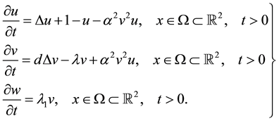
A reaction diffusion type mathematical model for growth of corals in a tank is proposed in [11] [12] con- sidering the nutrient polyps interaction. This model is derived based on the model appear in [8] . The non- dimensionalized version of this mathematical model takes the form:
 (1)
(1)
Here, u and v are vertically averaged nondimensionalized concentrations of dissolved nutrients (foods of coral polyps) and aggregating solid material (calcium carbonate) on the coral reefs respectively. , d,
, d,  and
and  are positive constants. The local and global stabilities of the solutions of the corresponding system of ordinary differential equations
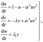 (2)
(2)
are discussed in [11] . Turing type instability analysis and patterns formation behavior of the model (1) subject to the boundary conditions
 (3)
(3)
are discussed in [12] . Here  denotes the gradient operator and
  denotes the outward unit normal vector to the domain boundary
 .
.
1.1. Constant Solutions (Steady States)
There are three constant solutions (homogeneous steady sates)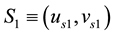 ,
,  and
and
 for the system (1). Here
 ,
,  ,
,  ,
,  ,
, ![]() and
and ![]() for
for![]() .
.
1.2. Stationary Problem
In this article, the existence of the stationary solutions of the system (stationary problem corresponding to the system (1)):
![]() (4)
(4)
subject to no-flux boundary conditions (3), is discussed.
The main result presented in this article is the existence of non-constant positive solutions. These existence results are proved based on the Priori estimates and Topological Degree theory [13] - [15] .
2. Priori Estimates
In this section we obtain estimates for the upper and lower bounds for the stationary solutions of the system (4). This boundedness property can be expressed as the following theorem:
Theorem 1. Let ![]() be any solution of (4) except
be any solution of (4) except![]() . Then there exists a constant C such that
. Then there exists a constant C such that
![]()
for![]() , where
, where![]() .
.
Our main aim here is to prove the above theorem. In order to prove this, let us first prove following results:
Lemma 1. Let ![]() be any nontrivial solution of (4). Then
be any nontrivial solution of (4). Then ![]() and
and ![]() for
for![]() . Fur-
. Fur-
thermore, if![]() , then
, then ![]() for
for![]() .
.
Proof. Let![]() . Then applying maximum principle at
. Then applying maximum principle at ![]() we get
we get
![]() . That is,
. That is, ![]() , which implies
, which implies
![]() (5)
(5)
Therefore,![]() . Let
. Let![]() . Again applying maximum principle at
. Again applying maximum principle at ![]() we
we
get![]() . That is,
. That is, ![]() , which implies
, which implies![]() .
.
That is![]() . Since
. Since![]() , from the second equation of (4) we have
, from the second equation of (4) we have
![]() Applying strong maximum principle to the above equation we get
Applying strong maximum principle to the above equation we get ![]() in
in![]() , provided
, provided![]() . The proof is complete. □
. The proof is complete. □
Lemma 2. Assume that ![]() is any solution of (4). If
is any solution of (4). If![]() , then
, then ![]() for
for![]() .
.
Proof. Let![]() . Then
. Then
![]()
Also, ![]() on
on![]() . Then applying maximum principle we have
. Then applying maximum principle we have![]() , which implies the required inequality. □
, which implies the required inequality. □
Lemma 3. Assume that ![]() is any solution of (4). If
is any solution of (4). If![]() , then
, then ![]() for
for![]() .
.
Proof. Put![]() , Then
, Then
![]()
Since ![]() on
on![]() , the maximum principle gives the required inequality. □
, the maximum principle gives the required inequality. □
Lemma 4. Let ![]() be any solution for (4). Then there exist a constant
be any solution for (4). Then there exist a constant![]() , such that
, such that ![]() for
for![]() .
.
Proof. From lemma (1), we have
![]() (6)
(6)
From lemma (2) we get ![]() for all
for all ![]() From lemma (3) we get
From lemma (3) we get
![]() . Combining these two inequalities we have
. Combining these two inequalities we have ![]() (say). Then from (5) we have
(say). Then from (5) we have
![]() (7)
(7)
Therefore, ![]() for all
for all ![]() □
□
Lemma 5. Assume that ![]() is any solution of (4) except
is any solution of (4) except![]() . Then there exist a positive constant
. Then there exist a positive constant ![]() such that
such that ![]() for all
for all![]() .
.
Proof. The second equation of the system (4) can be written as ![]() in
in![]() , where
, where
![]() . From lemmas (1) and (3) we get
. From lemmas (1) and (3) we get ![]() and
and ![]() for any
for any![]() . Then
. Then ![]() Set
Set ![]() According to Harnack inequality [15] there
According to Harnack inequality [15] there
exists a parameter ![]() such that
such that
![]() (8)
(8)
Denote ![]() and
and![]() . Then applying maximum principle for the second equ-
. Then applying maximum principle for the second equ-
ation of (4), we have![]() . Since
. Since![]() , we get
, we get
![]() (9)
(9)
From the inequalities (8) and (9) we get
![]() for all
for all![]() . That is
. That is ![]() for all
for all![]() ,
,
where![]() . □
. □
Proof of Theorem (1): From lemma (3) we have, ![]() ,
, ![]() and, from
and, from
lemma (5) we have ![]() for all
for all![]() . Set
. Set
![]() (10)
(10)
Then we have ![]() □
□
3. Existence of Non Constant Stationary Solutions
In this section we investigate the existence of non-constant solutions to (4). For this, the degree theory for compact operators in Banach spaces [15] [16] are used as the main mathematical tool. Define the spaces ![]() and Y as follows:
and Y as follows:
![]()
![]() and
and ![]() Here C is the con-
Here C is the con-
stant defined in Equation (10) and ![]() is any solution of the system (4). Set an auxiliary parameter
is any solution of the system (4). Set an auxiliary parameter ![]() for
for![]() , where M is a large constant to be determined. Let
, where M is a large constant to be determined. Let ![]() denote any constant solution of the system (4). Linearizing the system (4) when
denote any constant solution of the system (4). Linearizing the system (4) when ![]() at S takes the form:
at S takes the form:
![]() (11)
(11)
Denote
![]()
and
![]()
Thus,![]() . Then (4) and (11) can be written as
. Then (4) and (11) can be written as
![]() (12)
(12)
respectively. Define![]() , and
, and ![]() That is
That is ![]() is a compact perturbation of the identity operator. According to the definition of
is a compact perturbation of the identity operator. According to the definition of ![]() there is no fixed point of T on the boundary
there is no fixed point of T on the boundary![]() . Thus,
. Thus, ![]() is a positive solution of (12) if and only if
is a positive solution of (12) if and only if ![]() So, the Leray-Schauder degree
So, the Leray-Schauder degree ![]() is well defined. Furthermore, we have
is well defined. Furthermore, we have ![]()
The index of ![]() at
at ![]() is defined as
is defined as
![]()
where ![]() is the number of negative eigenvalues of
is the number of negative eigenvalues of![]() .
.
Lemma 6. The eigenvalues, ![]() of
of ![]() are given by the equation
are given by the equation
![]() (13)
(13)
where ![]() and
and ![]() Here p and q are the trace and determinant of the matrix A respectively and
Here p and q are the trace and determinant of the matrix A respectively and ![]()
![]() are the positive eigenvalues of the eigenvalue problem
are the positive eigenvalues of the eigenvalue problem
![]() (14)
(14)
such that![]() . Also the discriminant D of (13) is given by
. Also the discriminant D of (13) is given by
![]()
Proof. The eigenvalues ![]() of
of ![]() satisfies
satisfies
![]()
This implies
![]() (15)
(15)
By simplifying we get
![]()
This implies
![]()
where ![]() and
and ![]() The discriminant of (13) is
The discriminant of (13) is
![]()
![]() □
□
Now we consider the cases ![]() and
and ![]() separately.
separately.
3.1. The Case α > 2λ
In this case there are two constant fixed points of ![]() in
in ![]() which are
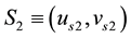
which are ![]() and
and ![]() . Now we deal with the case
. Now we deal with the case![]() . Let
. Let![]() ,
, ![]() and
and ![]() be corresponding P value, Q value and the discriminant of (13) respectively. Also let
be corresponding P value, Q value and the discriminant of (13) respectively. Also let ![]() and
and ![]() be the corresponding p and q values.
be the corresponding p and q values.
3.1.1. The Case ![]()
The solutions for ![]() of the Equation (13) can be written as
of the Equation (13) can be written as
![]() and
and
If ![]() then
then ![]() and
and![]() . It can be shown that
. It can be shown that![]() . That is, if
. That is, if ![]() then only one negative solution exists for (13). It follows that if
then only one negative solution exists for (13). It follows that if ![]() is negative we can find
is negative we can find
![]() ,
, ![]()
![]() such that
such that![]() . Therefore,
. Therefore, ![]()
3.1.2. The Case ![]()
Next we deal with the case![]() . Let
. Let![]() ,
, ![]() and
and ![]() be corresponding P value, Q value and the corresponding discriminant of (13). Also let
be corresponding P value, Q value and the corresponding discriminant of (13). Also let ![]() and
and ![]() be the corresponding p and q values. In this case we can find
be the corresponding p and q values. In this case we can find![]() ,
, ![]() such that
such that ![]() is negative when
is negative when![]() . Therefore there are exactly one neg- ative solutions for the corresponding Equation (13) when
. Therefore there are exactly one neg- ative solutions for the corresponding Equation (13) when![]() . Therefore
. Therefore![]() . Also,
. Also,
![]() (16)
(16)
Theorem 2. Assume that![]() ,
, ![]() and
and ![]() are satisfied. If
are satisfied. If ![]() is even, then (4) has at least one positive nontrivial solution.
is even, then (4) has at least one positive nontrivial solution.
Proof. Homotopy invariance property show that
![]()
By setting ![]() as sufficiently large constant we get
as sufficiently large constant we get![]() ,
,![]() . Therefore,
. Therefore,
![]() (17)
(17)
Also, we have
![]() (18)
(18)
The relations (17) and (18) contradict the homotopy invariance property for![]() ,
,![]() . Thus the proof is complete. □
. Thus the proof is complete. □
3.2. The Case α = 2λ
In this case the constant fixed point of ![]() in
in ![]() is uniquely determined by
is uniquely determined by![]() . The Leray- Schauder index at this point is:
. The Leray- Schauder index at this point is:
![]()
where ![]() is the number of real negative eigenvalues (counting algebraic multiplicity) of
is the number of real negative eigenvalues (counting algebraic multiplicity) of![]() .
.
In this case ![]() and
and![]() . Then,
. Then,
![]()
and
![]()
If![]() :
:
Then ![]() and
and![]() . Therefore, if
. Therefore, if![]() , then
, then![]() . That is if
. That is if![]() , there is
, there is
exactly one negative solution for (13). No negative solutions for (13) if ![]()
If![]() :
:
In this case, Q is negative if![]() . Then there is exactly one negative solution for (13).
. Then there is exactly one negative solution for (13).
Let ![]() be the number of
be the number of![]() , satisfying
, satisfying![]() . Then,
. Then,![]() .
.
Theorem 3. Assume that![]() . If
. If ![]() is odd, then (4) admits at least one positive non-constant solution.
is odd, then (4) admits at least one positive non-constant solution.
Proof. From the Homotopy invariance property we have
![]()
Suppose that (4) has no non-constant solutions if![]() . Also
. Also
![]()
provided ![]() is sufficiently large. On the other hand
is sufficiently large. On the other hand
![]()
These two relations contradict the homotopy invariance property for![]() ,
,![]() . Thus the proof is complete. □
. Thus the proof is complete. □
4. Discussion
Stationary problem corresponding to a model mathematical model for formation of coral patterns is considered. We have proved the existence of non-constant positive solutions of the stationary problem (4). Existence of non- constant solutions to the stationary problem gives a guarantee for the existence of spatially variant time invariant solutions to the proposed reaction-diffusion system. In other words, the solution of the system reaches a steady state with spatial patterns. This is a physically important feature which gurantees the the existence of stable coral patterns of the system.