Movement and Heat Transfer of Particles in Inhomogeneous and Nonisothermal Rapidly Oscillating Fluid Flow ()
1. Introduction
Fluid or gas turbulent flows with particles or droplets widely occur in natural phenomena and are intensively used in various technical applications. Owing to the slip condition for fluid phase intensity of velocity and temperature fluctuations has substantial heterogeneity. In this case, the additional force of migration occurs, and consequently the particle drifts to a channel wall [1] -[4] . Temperature fluctuations and migration of particle to the wall lead to an additional heat flux. Magnitude of these effects is determined by dynamic and thermal relaxation times of the particle and integral time scale of turbulence. In theoretical studies of two-phase turbulent flows migration force is included on the basis of the probability density function [2] -[4] . The main purpose of the present work is to investigate the physical mechanism of inertial particles drifting in the inhomogeneous turbulence. We use a simple model in which the fluctuations of velocity and temperature of the liquid phase are approximated by periodic oscillations. The amplitude of the oscillations is inhomogeneous in space. For separation of a particle motion into fast and slow components is involved the method of averaging developed by Krylov and Bogolyubov [5] -[7] . Closed system of ordinary differential equations for particle trajectories and temperature averaged over the oscillation period was derived. It is shown that migration force is directed toward reducing the amplitude of the velocity fluctuations of liquid phase. Effect of particles drift reaches a maximum value for particles with dynamic relaxation time compared with the oscillation period.
For a linear dependence of amplitude of velocity and temperature oscillation on the distance from a wall, the analytical solution was obtained. Combined influence of gravity and migration forces on a particle trajectory was studied. The results of numerical integration of complete system of differential equations of dynamics and temperature of particles are in satisfactory agreement with the calculations obtained by analytical formulas.
2. Basic Equations
For the purpose of compactness of the presentation and elucidate the physical meaning of obtained results, we consider one-dimensional case. We study oscillating field of fluid velocity in the direction normal to the solid wall (see Figure 1). Coordinate axis  is directed along the normal to the wall. Fluid velocity
  and gravity vector
  are parallel to the normal.
Differential equations for a particle velocity , coordinate
  and temperature
  have the form
 , (1)
, (1)
 , (2)
, (2)
Here  is fluid temperature;
  are dynamic and temperature relaxation times of the particle [4]
 .
.
Here  are densities of fluid and particle material;
  are heat capacities of fluid and particle material;
  is particle diameter;
  is thermal diffusivity;
  is coefficient of aerodynamic drag;
  is Nusselt number of the particle.
Generally, the drag coefficient and Nusselt number depends on the particle Reynolds number
 (
( is kinematic viscosity coefficient of fluid phase). In the analysis we assume drag coefficient and Nusselt number as constant. This approximation corresponds to the Stokes flow regime. For Stokes flow regime
 ,
,  and the ratio of dynamic and temperature time scales of the particle is equal
 where
where  is Prandtl number of the fluid.
It can be seen, that the distinction in the thermo-physical properties of liquid and material of particle leads to different values of thermal and dynamic relaxation times.
The initial conditions for the system of equations (1) and (2) have the form
 . (3)
. (3)
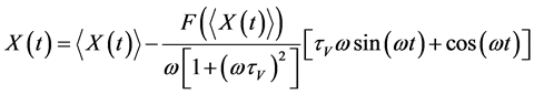
Dependences of velocity and temperature of fluid on the distance from the wall (see Figure 1) are defined as
 . (4)
. (4)
The main purpose of this manuscript is to show that in an inhomogeneous, rapidly oscillating non-isothermal fluid flow appear migration force and an additional heat flux connected with inertia of the particles.
3. The Averaging Method
Equation (1) is reduced to the single equation for displacement of a particle
 . (5)
. (5)
To solve the equation (5) we involved the Krylov-Bogolyubov method of averaging [4] -[6] . Displacement and temperature of particles composed of slow averaged components ,
,  and fast oscillations of displacement
  and temperature
 .
.
By averaging over the oscillation period  we obtain the following expressions
 .
.
Fluctuations of particle coordinate is substantially lesser than the averaged displacement .
.
Functions representing the amplitude of velocity and temperature of carrier fluid (4) along the particle trajectory are written in the form of an expansion in the sense of small oscillations of the particle coordinate
 .
.
With these formulas and the equation for temperature (2) and coordinate (5) of the particle take the form
 (6)
(6)
 (7)
(7)
Fluctuations of velocity and temperature of a particle represented as
 . (8)
. (8)
Correctness of the above presentations are illustrates in Appendix. Period of oscillation  is substantially less than the time scale of variation of averaged parameters for the particle. Time derivatives of velocity and temperature fluctuations of the particle have the form
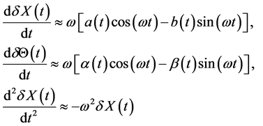
Upon substituting these expressions into the Equation (6) we write down
 (9)
(9)
For particle temperature (7) following equation is rewritten
 (10)
(10)
Unknown coefficients  are obtained from the equations (9) and (10) taking into account the orthogonally of functions
  and
and  on the temporary interval
 ,
,
 .
.
Equations (9) and (10) is multiplied sequentially by functions ,
,  and integrated over the period of oscillation
 . As a result, from Equation (9) we obtain expressions for the coefficients
 .
.
From equation (10) we obtain expressions for the coefficients 
 ,
,
 .
.
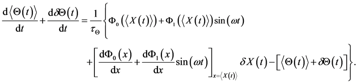
After averaging the equations (9) and (10) over the period of oscillation we obtain the following equations for averaged velocity and temperature of the particle
 , (11)
 . (12)
From the equations (11) and (12) is seen that in homogeneity in amplitude of velocity and temperature fluctuations of carrier fluid leads to migration force and an additional heat transfer for particles. The drift velocity in equation (11) is proportional to derivative of the square of amplitude of fluid velocity fluctuations and directed toward reducing intensity of fluctuations . From equation (12) one can notice that at inhomogeneous temperature of fluid on the particle acts additional cooling heat flux for
 .
.
It follows from the equation (11) that, for particles of low inertia  additional migration force and additional heat flux disappears. Value of migration force and additional heat flux is also reduced for particles with high inertia
 . Migration force is maximal for particles with a relaxation time
 .
.
Actual coordinate and velocity of particles are calculated based on the following algebraic equations
 , (13)
 . (14)
Actual temperature of particle is
 . (15)
From the formulas (3) it is follow the initial conditions for the averaged velocity, temperature and particle coordinate
 ,
,
 ,
,
 .
.
4. Linear Dependence of Velocity and Temperature Amplitudes
Consider the analytical solution for the case of linear dependence of amplitude of fluctuations of velocity and temperature of liquid with the distance from the wall (see Figure 1)
 .
.
4.1. Solution of the Equations for a Particle Velocity and Coordinate
In considered case the equation for averaged particle coordinate has the following form
 .
.
Solution of the last equation can be written as
Constants  is founded from the initial conditions (3)
 .
.
Expression for actual coordinate of particle follows from (13)
 .
.
In this considered special case equation for averaged particle velocity has the form
 .
.
Solution of this equation is
 .
.
Initial values for the averaged coordinate and velocity of a particle are
 .
.
Actual velocity of a particle follows from expression (14)
 .
.
4.2. Solution of Equation for a Particle Temperature
Equation for averaged temperature of a particle follows from equation (12) and has the form
 . (16)
Initial value of average temperature of a particle is equal
 .
.
Solution of Equation (16) represented
 .
.
By substituting in the above integral expression for the averaged particle displacement , we find out the following formula
 .
.
Formula for actual temperature of a particle follows from expression (15) and takes the form

5. Calculation Results
We give comparison of the results of analytical research with the data of direct numerical calculation of the system of equations (1) and (2). As dimensionless variables we used Stokes number , dimensionless temporary variable
  and dimensionless coordinates
 ,
, . Dimensionless gravity acceleration is
  and dimensionless thermal relaxation time is
 .
.
Figure 2 illustrates a satisfactory agreement between results of calculations using analytical formulas from the previous paragraph and numerical integration the ordinary differential equations (1) and (2). Migration of particles towards the wall is a result of its inertia. One can see that particle drifts to the wall. This effect can be explained as follows. On the one hand, a particle leaves the region with high level of velocity fluctuations and enters in a region with low level. On the other hand, viscous resistance leads to loss of kinetic energy of the particle. Particle due to its inertia cannot return to the region with a higher level of velocity fluctuations.
The Figure 3 illustrates the effect of preferential concentration of particles at some distance from the wall when the gravity force is directed along the normal to the wall (see Figure 1). Unlike the case ( ), the particle periodically fluctuates at a certain distance from the wall.
The Figure 4 presents a satisfactory agreement between the results of numerical integration of differential equations (1) and (2) and calculations using analytical formulas for the particle temperature. Figure represent the alteration of temperature with time (a) and change the particle temperature along its trajectory (b). The particle drift toward the wall and its temperature decreases.
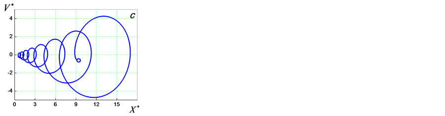
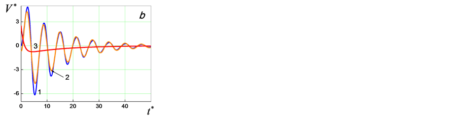
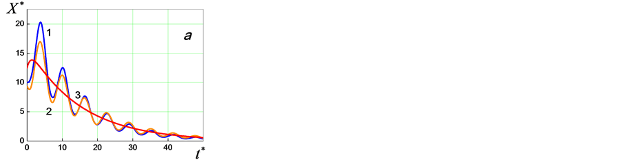
Figure 2. Dimentionless coordinate (a), velocity (b) and phase diagram (c) for St = 1: 1—analytical formulas for actual coordinate and velocity of a particle; 2—solution of ODE; 3—average trajectory.
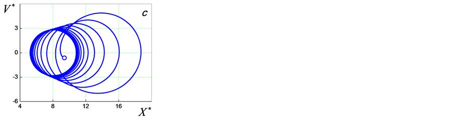

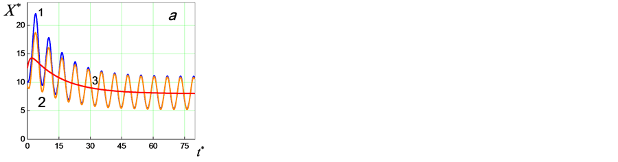
Figure 3. Nondimensional coordinate (a), velocity (b) and phase diagram (c) for St = 1, g* ≠ 0. Other designations as in Figure 2.


Figure 4. Nondimensional temperature (a) and phase diagram (b) for St = 1, . Other designations as in Figure 2.
6. Conclusions
Simple model of a particle motion and heat transfer in inhomogeneous field of fluctuating velocity and temperature of fluid was suggested. The proposed model reflects the main features of the turbulent flow near the wall. For separation of the fast and slow components of velocity and temperature fluctuations of a particle averaging method of Krylov-Bogolyubov was used.
Physical interpretation of migration force and additional feat flux in inhomogeneous rapidly oscillating velocity and temperature of fluid phase is established. It is shown that the force of migration and additional heat flux disappear for low inertia particles and decrease with increasing particles Stokes number.
For a linear dependence of the amplitude of velocity and temperature fluctuations on the distance to the wall analytical solutions was found. The results of numerical solution of the system of equations of motion and heat transfer of a particle are in satisfactory agreement with the calculations by analytical formulas.
The possibility of formation regions with preferential concentration of particles in a gravitational field and in inhomogeneous velocity fluctuations is illustrated.
Acknowledgements
This work was supported by RFBR grant14-08-00970.
Appendix
Here we will illustrate the correctness of presentation of velocity and temperature fluctuations in the form (8). For a homogeneous fluid velocity in dimensionless variables we have the equation for a particle velocity
 .
.
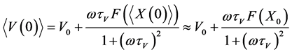
Particle velocity with the initial condition is
 .
.
For a sufficiently long interval of time , we obtain the following expression
 .
.
From above expression we see that stationary amplitude of oscillation decreases with increasing Stokes number.
The Figure A1 illustrates process of reaching the stationary regime for particle velocity fluctuations.
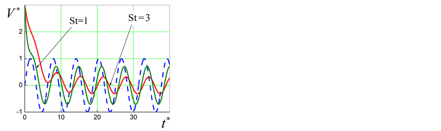
Figure A1. Particle velocity in versus of time. Dached line shows velocity oscillation of fluid phase.