Lie Symmetries, 1-Dimensional Optimal System and Optimal Reductions of (1 + 2)-Dimensional Nonlinear Schrödinger Equation ()
1. Introduction
Inspired by Galois’ theory, Sophus Lie developed an analogous theory of symmetry for differential equations. Lie’s theory led to an algorithmic way to find special explicit solutions to differential equation with its admitted symmetry. These special solutions are called group invariant solutions and they constitute practically every known explicit solution to the systems of non-linear partial differential equations (PDEs) arising in mathematiccal physics, differential geometry and other areas. These group-invariant solutions are found by solving a reduced system of differential equations involving fewer independent variables than the original system. The reduced system is obtained through reducing the underline system by using its admitted Lie symmetry. Hence, it is critical to solve the invariant solutions that one finds all the symmetries of the original system. On the other hand, the algebra properties of the Lie algebra corresponding to the Lie symmetry group of a PDE show some essential nature of the solutions of the PDE. For example, from the optimal structure of the Lie algebra, one can solve optimal set of invariant solution to the PDE, which is critical to distinguish different classes of invariant solutions of the PDE.
Generally, an optimal system of s-parameter subgroups of a Lie algebra is a list of conjugacyin equivalent s-parameter subgroups with the property that any other subgroup is conjugate to precisely one subgroup in the list. Correspondingly, a list of s-parameter subalgebras forms an optimal system if every s-parameter subalgebra of the Lie algebra is equivalent to unique member of the list under some element of the adjoint representation set. The optimal system of a Lie algebra provide the optimal classification of various different dimensional subalgebras. For a PDE, the optimal system of the Lie algebra admitted by the PDE provides the optimal classification of invariant solutions of the PDE under its Lie symmetry group.
In this paper, we plan to consider the (1 + 2)-dimensional nonlinear Schrödinger equation (NLSE) with cubic nonlinearity [1]
 (1)
(1)
where  is a complex function and
  is a non-zero real parameter. This equation occurs in various chapters of physics, including nonlinear optics, superconductivity, quantum mechanics and plasma physics [2] . The cubic nonlinearity is the most common nonlinearity in applications. It arises as a simplified model for studying Bose-Einstein condensates, Kerr mediain nonlinear optics freak waves in the ocean (see [3] and references therein).
For the NLSE (1), many researchers’ work mostly concentrated on obtaining exact or approximate solutions. The classical symmetry reductions and some similarity solutions of the (1) are given in [1] by Lie symmetry method. Its some approximate solutions are obtained in [3] with applying the differential transform method. The 1-soliton solution of (1) has been obtained in [4] . Reliable analysis for the (1 + 1)-dimensional NLSE with power law nonlinearity has been investigated by Wazwaz in [5] . Some soliton and periodic solutions of (1 + 2)-dimensional NLSE (1) are constructed in [6] . However, the algebra properties of the Lie algebra admitted by the NLSE (1) such as optimal system of the Lie algebra, have not been studied so far.
We will construct optimal systems of the Lie algebra of the both NLSE (1) and its first reduction systems under their admitted Lie symmetry groups respectively. Furthermore, we derive twice reductions of NLSE (1) with respect to the obtained optimal system. Consequently, we show the NLSE (1) can be reduced to ordinary differential equations which yields exact solutions of the equation. The outline of the article is following. In section 2, the 9-dimensional classical Lie algebra  of (1) is given by characteristic set algorithm proposed in In section 3, 1-dimensional optimal system of the Lie algebra derived by using the algorithm given in [7] . In section 4, the first reductions with respect to the obtained optimal system of the equation are studied by means of Lie’s method of infinitesimal transformation. In Section 5, the optimal system of 6-dimensional Lie algebra
  of a first reduced equations of the NLSE (1) obtained in Section 4 are given. Consequently, we obtain a twice reduction of the original equation (1). In Section 6, some exact invariant solutions of the NLSE (1) are obtained by combining the twice reductions procedure using invariant method given in [8] . Concluding remarks are given in Section 7.
2. Lie Symmetry of the Equation (1)
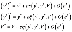
In this section we present the generators of the Lie algebra corresponding to classical symmetries of the NLSE (1). Let theone parameter Lie group of infinitesimal transformations in  given by
 (2)
(2)
where  is the group parameter. The corresponding generator of the Lie algebra is
 (3)
(3)
For fitting the algorithm and software in [9] , transform the NLSE (1) to real case by transforming , where
  and
and  are real function. For this transformed system, using characteristic set algorithm given in [9] , we find the simplified determining equations for generator

are as follows
 ,
,  ,
,  ,
,
 ,
,  ,
,  ,
,  ,
,
 ,
,  ,
,  ,
,  ,
,  ,
,  ,
,
 ,
,  ,
,  ,
,  ,
,  ,
,
 ,
,  ,
,  ,
,  ,
,
 ,
,  ,
,  ,
, .
.
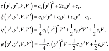
Solving the above system of PDEs, we obtain:

where  are arbitrary constants.
Therefore the infinitesimal generators of the transformed real form equations are given by
 ,
,  ,
,  ,
,  ,
,
 ,
,  ,
,  ,
,
 ,
,
 .
.
These are equivalent to generators for Lie algebra of NLSE (1) obtained by transforming ,
,  ,
,  It spans 9-dimensional Lie algebra
  of admitted by NLSE (1). The commutation relations of (4) are given in the following Table1 It is fundamental to constructing the optimal system of
  spanned by (4).
 ,
,  ,
,  ,
,  ,
,
 ,
,  ,
,  , (4)
, (4)
 ,
, .
.
The commutation relations of the basis is given in the following Table1
3. 1-Dimensional Optimal System of 
In this section we present a 1-dimensional optimal system of the algebra  obtained in Section 2 spanned by (4).
The problem of finding an optimal system of subalgebra of a Lie algebra is a subalgebraclassification problem. Unfortunately,this problem can still be quite complicated and has no efficient method to use. For 1-dimensional subalgebras, this classification problem is essentially the same as the problem of classifying the orbits of the adjoint representation, since each 1-dimensionalsubalgebra is determined by a nonzero vector in the algebra. Essentially, this problem is attacked by the naive approach of taking a general element  in the algebra and subjecting it to various adjoint transformations so as to “simplify” it as much as possible.
Now, in our case, given a nonzero vector  in algebra spanned by (4). The vector corresponds to the vector
 . Our task is to simplify as many of the coefficients
  being zero as possible through applicationof adjoint maps on
  and find its equivalent one.
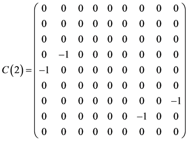
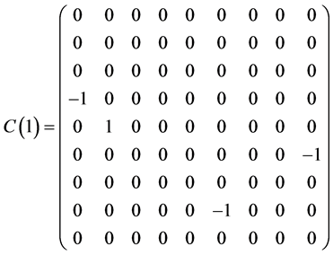
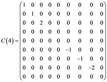
Here we use the matrix method given in [7] to determine an optimal system of 1-dimmensional subalgebra of . Thealgorithm is given by following steps.
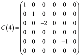
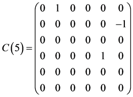
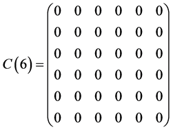
Step 1. Determine structure constants matrix  by formula

where  is structure constants given in commutator table 1.
Step 2. Calculate adjoint matrix  by definition.

Step 3. Simplify the vector  as much as possible by applying
  on k and obtain equivalent one of
 .
.
In the Following, we construct the optimal system of  by following above the steps.
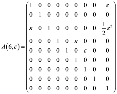
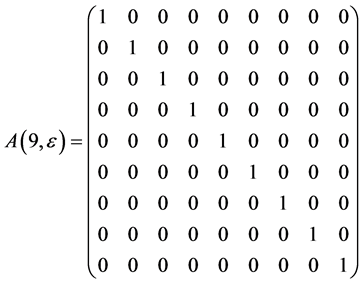
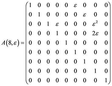
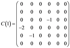
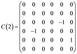
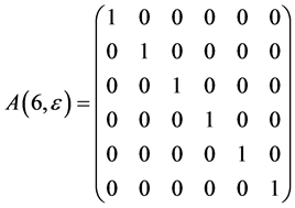
As the commutator table 1 showing, we have the structure constants matrices for the  areas follows

Table 1 . Commutation table for the generators of the Lie algebra
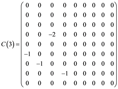
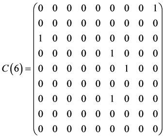
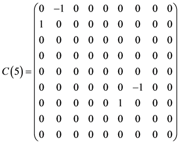
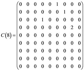
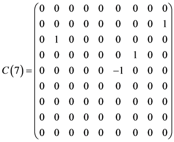
and
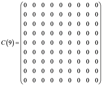
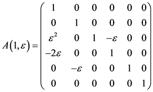
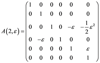
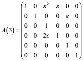
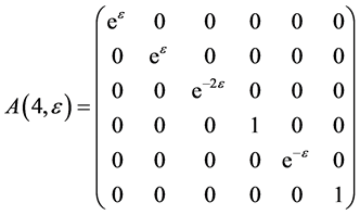
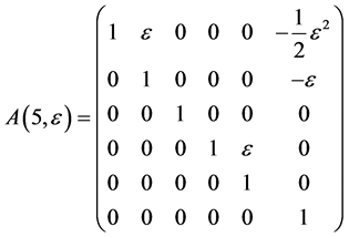
The exponentiation of the matrices  leads to adjoin matrix
  which are as follows
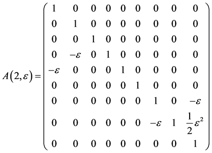
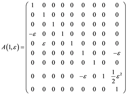
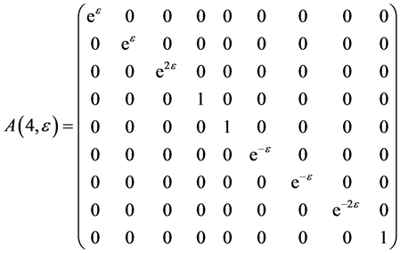
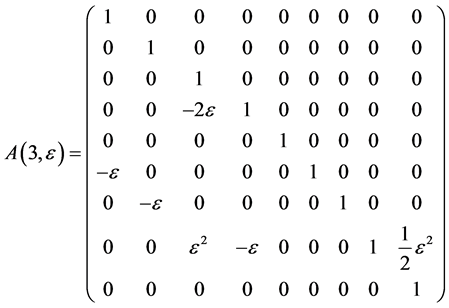
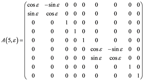
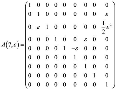
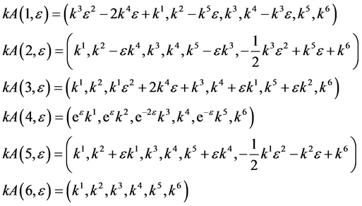
Hence, the vector  is transformed by the matrices
  is as follows
 ,
,
 ,
,
 ,
,
 ,
,

 ,
,
 ,
,
 ,
,
 .
.
In order to obtain the optimal system, we solve  as simple as possible from the above transformations.
If , by setting
 ,
,  ,
,  ,
,  ,
,  , the coefficients
  and
and  are vanished. By scaling, we can suppose
 , Hence X is equivalent to
 , where we use a, b, c and q to denote the arbitrary constants.
If  and
and , by setting
 ,
,  ,
,  ,
,  ,
,  coefficients
  and
and  are vanished. By scaling, we can suppose
 。 Hence
  is equivalent to
 .
.
If  and
and , by setting
 ,
,  ,
,  , coefficients
and  are vanished. By scaling, we can suppose
 . Hence
  is equivalent to
 .
.
If  and
and , by setting
 ,
,  ,
,  coefficients
  and
and  are vanished. By scaling, we can suppose
 . Hence
  is equivalent to
 .
.
If  and
and , by setting
 ,
,  ,
, 
 , coefficients
  are vanished. By scaling, we can suppose
 . Hence
is equivalent to .
.
If  and
and , by setting
 ,
,  ,
,  coefficients
  are vanished. By scaling, we can suppose
 . Hence
  is equivalent to
 .
.
If  and
and  by setting
 ,
,  ,
,
 , coefficients
  are vanished. By scaling, we can suppose
 . Hence
  is equivalent to
 .
.
If  and
and , by scaling, we can suppose
 . Hence
  is equivalent to
 .
.
If , by scaling, we can suppose
 . Hence
  is equivalent to
 .
.
Therefore the set of generators
 (5)
(5)
is consisted of the optimal system of 1-dimensional subalgebra of the algebra  of the NLSE (1), where
  and
and  are arbitrary constants.
4. Reductions of NLSE (1) with (5)
In this section we give a classification of symmetry reductions of NLSE (1) by using (5).
The reduction in this section require lengthy computations and do not follow a standard algorithmic procedure, so it would be difficult to reproduce them using software. We will introduce the details for the case
 and the remaining ones can be reproduced in a similar manner.
The differential invariants (and hence the similarity variables) for the generator can be determined by solving the characteristic system
 (6)
(6)
Solving this system, one obtains invariant (similarity) variables are as follows
 ,
,
 ,
,
 .
.
Hence let
 (7)
(7)
and substitute (7) into the equation (1) which yields the first reduced system of the NLSE (1)
 (8)
(8)
In the same manner, we can obtain the additional reductions of (1) with using other subalgebras in (5) which are listed in Table2 The last column shows the cases of similarity variables. Here


Table 2. The first reductions of equation (1) by optimal system (5).


5. Reductions of NLSE (1) with (5)
The equations obtained in Table 2 can be reduced further in the similar way in last section, consequently, we obtain second time reductions of NLSE (1). We take the first equation (the reduced one of (1) by  or
or ) in Table 2
 (9)
(9)
as example. This is a nonlinear “1 + 1” Schrödinger equation.
5.1. Lie Symmetry of the Equation (9)
In this section we present all symmetries of equation (9). To obtain the Lie group symmetries of equation (9)we consider the one parameter Lie group of infinitesimal transformations in  given by
where  is the group parameter. The corresponding generator of the Lie algebra of the group symmetry is

For fitting the algorithm and software in [9] , we transform the (9) to real case by transformation  where
where  and
and  are real function. For this transformed system, we find the generator

for its Lie symmetry group. The simplified determining equations are
 ,
,  ,
,  ,
,  ,
,  ,
,
 ,
,  ,
,  ,
,  ,
,  ,
,  ,
,
 ,
,  ,
,  ,
, .
.
After solving the above system of PDEs, we have
Here  are constants.
Therefore the symmetry algebra generators are
 ,
,  ,
,  ,
,
 ,
,  ,
, .
.
By transformation ,
,  ,
,  , the 6-dimensional Lie algebra
  of (9) is spaned by the set of generators
 (10)
(10)
The commutation relations of the basis is given in the following Table3
5.2. 1-Dimensional Optimal System of the 
This section presents a optimal system of 1-dimensional subalgebras of the symmetry algebras  obtained in Section 5.1. As above section, we have
 ,
,  ,
,  ,
,
 ,
,  ,
, .
.
The exponentiation of the matrices  are obtained as follows
Table 3 . Commutator for (10).
 ,
,  ,
,
 ,
,  ,
,
 ,
, .
.
For the nonzero generator , the vector
  is transformed by the matrices
  as follows
In order to get the optimal system, we need to transform  as simple as possible. This is done by following deduction.
If  by setting
 ,
,  and
and , the coefficients
  and
and  are vanished. By scaling, we can suppose
 . Hence
  is equivalent to
 .
.
If  and
and  by setting
 ,
,  ,
,  and
and , the coefficients
 ,
,  and
and  are vanished. By scaling, we can suppose
 . Hence
  is equivalent to
 .
.
If  and
and  by setting
 ,
,  ,
,  and
and , the coefficients
  and
and  are vanished. By scaling, we can suppose
 . Hence
  is equivalent to
 .
.
If  and
and  by setting
 ,
,  and
and , the coefficient
  is vanished. By scaling, we can suppose
 . Hence
  is equivalent to
 .
.
If  and
and  by setting
  and
and . By scalingwe can suppose
 . Hence
  is equivalent to
 .
.
If  and
and , by scaling, we can suppose
 . Hence
  is equivalent to
 .
.
Therefore the set of generators
 (11)
(11)
is consist of the optimal system of 1-dimensional subalgebra of the symmetry algebra of equation (9),where ,
,  and
and  are arbitrary constants.
5.3. 1-Dimensional Optimal System of the 
In this section we give a classification of symmetry reductions of PDE (9) with the optimal system of (11).
The equation (9) admits optimal system (11) obtained in Section 5.2.
Taking  as example to show the procedure of the reduction.
The differential invariants (and hence the similarity variables) for the generator can be determined by solving the characteristic system
 (12)
(12)
Solving this system, one obtains invariant (similarity) variables as follows

Hence let
 , (13)
which yields reduction of (9)
 .
.
This is the second reductions of (1), which is an ordinary differential equation.
In the same manner, we can obtain the second reductions of equation (9) with respect to other subalgebras of (11) whichare listed in Table4 For the equation reduced by  (the last equation in Table 2)
where


 (14)
(14)
we have the same reduction as (9).
For the equation reduced by  or
or  (the fifth equation in table 2)
 (15)
(15)
admits optimal system  and leads to the reductions which are listed in Table5
where
 ,
,  ,
,
 ,
, .
.
 ;
;
 ;
;
 ;
;
 .
.
Similarly, other equations in Table 2 also can be further reduced. Consequently, we obtain the twice reductions of (1) shown in Table6
where
 ,
,  ,
,  ,
,
 ,
,  ,
,  ,
, .
.
 ;
; ;
; ;
; ;
; ;
; ;
; ;
;
 ;
; ;
; ;
; ;
; ;
; ;
; .
.
Table 4. The further reductions of (9) with (11).
Table 5. The reductions for the subalgebras of equation (15).
 ;
;
 ;
;
 ;
;
 ;
; ;
;
 ;
;
 ;
; ;
; ;
; ;
;
 ;
; ;
;  Cannot get similarity variable;
Table 6. The rest reductions of the 2D-CNLS (1) by optimal system (6).
 Cannot get similarity variable;
 ;
;  Cannot get similarity variable;
 ;
; ;
;
 ;
; .
.
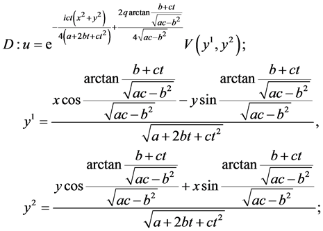
6. Some Exact Invariant Solutions of PDE (1)
In Table 4, we have
 (16)
(16)
Transform the (16) to real case by transformation , where W and
  are real functions, we find the simplified
 (17)
(17)
 (18)
(18)
Dividing equation (17) by equation (18), we obtain

which yields
 (19)
(19)
where , c is arbitrary constant. Substituting (19) to (18), it has general solutions
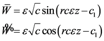
Therefore
 (20)
(20)
In the same manner, solving the equation

in Table 4, we have solution

In the same manner, solving the equation in Table 5

one has solution

These solutions  yield exact solutions of (1) through connection with
 , (20) and (7).
7. Conclusion
The 1-dimensional optimal system of the Lie algebra of 2D-CNLS equation has been constructed by matrix form methodand twice reductions of the equation by the optimal system are given. Consequently, some exact invariant solutions of theequation are formed by symmetry method.
Acknowledgements
This research was supported by the Natural science foundation of China (NSF), under grand number 11071159.
NOTES
*Corresponding author.